Area and Estimating with Finite Sums: Foundations of Integration

Area and Estimating with Finite Sums

Basic Area Formulas

Understanding the area of basic geometric shapes is foundational for calculus, especially when approximating areas under curves.

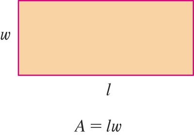
• Rectangle: The area is the product of its length and width.

• Formula: $A = l w$

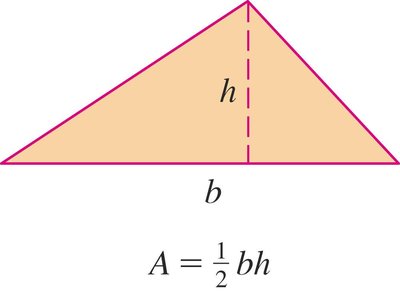
• Triangle: The area is half the product of its base and height.

• Formula: $A = \frac{1}{2} b h$

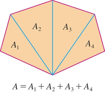
• Polygon: The area can be found by dividing the polygon into triangles and summing their areas.

• Formula: $A = A_1 + A_2 + \cdots + A_n$ (where $A_i$ are the areas of the constituent triangles)

Areas Under Curves and the Need for Approximation

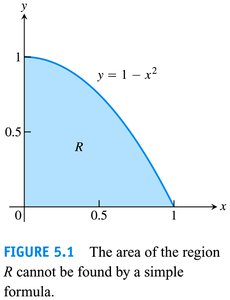
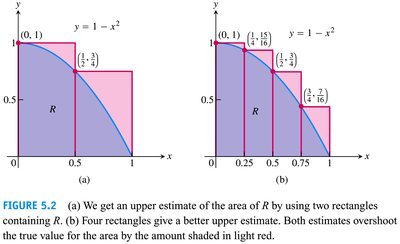
For many regions bounded by curves, such as the area under $y = 1 - x^2$ from $x = 0$ to $x = 1$, there is no simple geometric formula. Calculus provides tools to approximate and eventually compute these areas exactly.

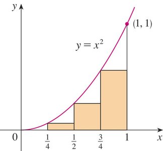
Rectangular Approximations (Riemann Sums)

To estimate the area under a curve, we can use rectangles:

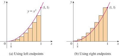
• Upper Sum: Rectangles overestimate the area (heights taken at the right endpoint or maximum value in each subinterval).

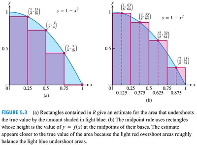
• Lower Sum: Rectangles underestimate the area (heights taken at the left endpoint or minimum value in each subinterval).

• Midpoint Sum: Heights are taken at the midpoint of each subinterval, often giving a better estimate.

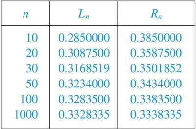
Numerical Results: Approximating Area

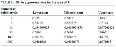
As the number of rectangles (subintervals) increases, the approximation improves. The table below shows how the lower, midpoint, and upper sums converge as the number of subintervals increases for the region under $y = 1 - x^2$.

Number of subintervals	Lower sum	Midpoint sum	Upper sum
2	0.375	0.6875	0.875
4	0.53125	0.617875	0.78125
16	0.634765625	0.6669921875	0.697265625
50	0.6566	0.6667	0.6766
100	0.66165	0.666675	0.67165
1000	0.6661665	0.66666675	0.6671665

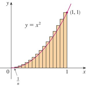
Generalization: Area as a Limit

The true area under a curve is defined as the limit of these sums as the number of rectangles approaches infinity and their width approaches zero. This is the foundation of the definite integral in calculus.

Sigma Notation and Summation Rules

Sigma Notation

Sigma notation is a concise way to write sums, especially those with many terms. The general form is:

• $\sum_{k=1}^n a_k$ means sum the terms $a_k$ as $k$ goes from 1 to $n$.

Examples and Algebraic Rules

Some common sums and their values:

The sum in sigma notation	The sum written out	The value of the sum
$\sum_{k=1}^5 k$	$1+2+3+4+5$	15
$\sum_{k=1}^3 (-1)^k k$	$(-1)^1(1) + (-1)^2(2) + (-1)^3(3)$	$-1+2-3=-2$
$\sum_{k=1}^3 \frac{k}{k+1}$	$\frac{1}{2} + \frac{2}{3} + \frac{3}{4}$	$\approx 1.92$
$\sum_{k=4}^5 \frac{k^2}{k-1}$	$\frac{4^2}{4-1} + \frac{5^2}{5-1}$	$\frac{16}{3} + \frac{25}{4} = \frac{139}{12}$

Algebraic rules for sums:

• Sum Rule: $\sum_{k=1}^n (a_k + b_k) = \sum_{k=1}^n a_k + \sum_{k=1}^n b_k$

• Difference Rule: $\sum_{k=1}^n (a_k - b_k) = \sum_{k=1}^n a_k - \sum_{k=1}^n b_k$

• Constant Multiple Rule: $\sum_{k=1}^n c a_k = c \sum_{k=1}^n a_k$

• Constant Value Rule: $\sum_{k=1}^n c = n c$

Special formulas:

• $\sum_{k=1}^n k = \frac{n(n+1)}{2}$

• $\sum_{k=1}^n k^2 = \frac{n(n+1)(2n+1)}{6}$

• $\sum_{k=1}^n k^3 = \left(\frac{n(n+1)}{2}\right)^2$

Summary

• Areas of basic shapes (rectangles, triangles, polygons) are foundational for calculus area approximations.

• For regions under curves, we use sums of rectangles (Riemann sums) to approximate area, improving accuracy as the number of rectangles increases.

• Sigma notation and summation rules provide a concise and systematic way to express and manipulate these sums.