Calculus I: Applications of Derivatives and Introduction to Integration

First Derivative Test and Concavity

Increasing and Decreasing Functions

The behavior of a function—whether it is increasing or decreasing—can be determined by analyzing its first derivative.

• Increasing Function: A function f(x) is increasing on an interval (a, b) if f'(x) > 0 for all x in that interval.

• Decreasing Function: A function f(x) is decreasing on an interval (a, b) if f'(x) < 0 for all x in that interval.

• To find intervals of increase and decrease, identify critical points (where f'(x) = 0 or f'(x) is undefined) and points of discontinuity.

First Derivative Test

The First Derivative Test helps determine the location of local maxima and minima by examining the sign changes of f'(x) around critical points.

• If f'(x) changes from positive to negative at x = c, then f(x) has a local maximum at x = c.

• If f'(x) changes from negative to positive at x = c, then f(x) has a local minimum at x = c.

Concavity and Inflection Points

Concavity describes the direction in which a function curves. Inflection points are where the concavity changes.

• Concave Up: f(x) is concave up on (a, b) if f''(x) > 0 on that interval.

• Concave Down: f(x) is concave down on (a, b) if f''(x) < 0 on that interval.

• Inflection Point: A point x = c where f(x) is continuous and the concavity changes (i.e., f''(x) changes sign).

Curve Sketching

Key Features for Sketching

To accurately sketch a function, analyze the following:

• Domain and Range

• x- and y-intercepts

• Horizontal and Vertical Asymptotes

• Intervals of Increase/Decrease

• Local Extrema

• Intervals of Concavity

• Inflection Points

L'Hôpital's Rule and Applied Optimization

L'Hôpital's Rule

L'Hôpital's Rule is used to evaluate limits that result in indeterminate forms such as 0/0 or ∞/∞.

• Theorem: If \lim\limits_{x \to a} f(x) = \lim\limits_{x \to a} g(x) = 0 or \pm\infty, and f(x) and g(x) are differentiable near a, then:

$\lim\limits_{x \to a} \frac{f(x)}{g(x)} = \lim\limits_{x \to a} \frac{f'(x)}{g'(x)}$

• Other indeterminate forms include ∞·0, ∞−∞, 1^∞, etc.

Applied Optimization

Optimization problems involve finding the maximum or minimum value of a function in a real-world context. The general process is:

1. Define variables for all changing quantities.

2. Write an equation for the objective to be optimized.

3. Express the objective in terms of a single variable.

4. Find critical points and use the First Derivative Test to determine extrema.

Antiderivatives and Areas Under Curves

Antiderivatives and Indefinite Integrals

An antiderivative of f(x) is a function F(x) such that F'(x) = f(x). The most general antiderivative is F(x) + C, where C is an arbitrary constant.

$\int f(x)\,dx = F(x) + C$

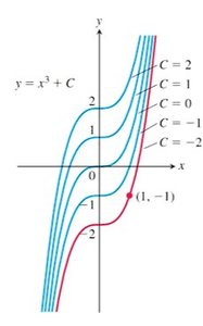
Initial Value Problems and Differential Equations

Solving a differential equation of the form dy/dx = f(x) involves finding an antiderivative. If an initial condition is given, such as y(x_0) = y_0, the solution is called an initial value problem.

Areas Under Curves and Riemann Sums

The area under a curve can be estimated using rectangles (Riemann sums). As the number of rectangles increases, the approximation becomes more accurate.

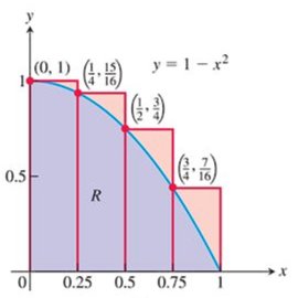
Riemann Sums and Sigma Notation

Sigma Notation and Summation Rules

Sigma notation is used to represent sums compactly:

$\sum\limits_{k=1}^n a_k = a_1 + a_2 + \ldots + a_n$

• Common summation formulas include:

$\sum\limits_{k=1}^n 1 = n$

$\sum\limits_{k=1}^n k = \frac{n(n+1)}{2}$

$\sum\limits_{k=1}^n k^2 = \frac{n(n+1)(2n+1)}{6}$

$\sum\limits_{k=1}^n k^3 = \left(\frac{n(n+1)}{2}\right)^2$

Types of Riemann Sums

There are three main types of Riemann sums, depending on which point in each subinterval is used to determine the rectangle's height:

• Left Endpoint: Uses the left endpoint of each interval.

• Midpoint: Uses the midpoint of each interval.

• Right Endpoint: Uses the right endpoint of each interval.

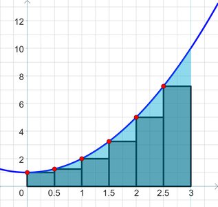
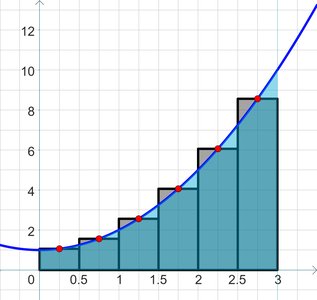
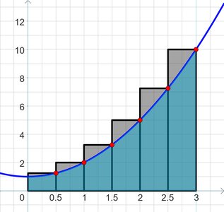
Improving Accuracy with More Rectangles

As the number of rectangles increases, the Riemann sum approaches the exact area under the curve.

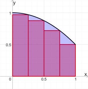
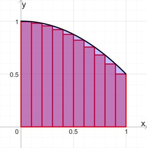
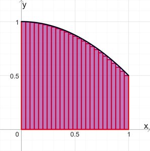
Definite Integrals and the Fundamental Theorem of Calculus (FTC)

Definite Integrals and Signed Area

The definite integral gives the signed area between a curve and the x-axis from x = a to x = b:

$\int_a^b f(x)\,dx$

• Area above the x-axis is positive; area below is negative.

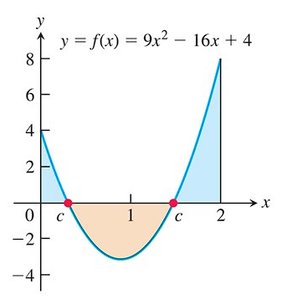
Properties of Definite Integrals

• $\int_a^a f(x)\,dx = 0$

• $\int_a^b k f(x)\,dx = k \int_a^b f(x)\,dx$

• $\int_a^b [f(x) \pm g(x)]\,dx = \int_a^b f(x)\,dx \pm \int_a^b g(x)\,dx$

• $\int_a^b f(x)\,dx + \int_b^c f(x)\,dx = \int_a^c f(x)\,dx$

• $\int_a^b f(x)\,dx = -\int_b^a f(x)\,dx$

Fundamental Theorem of Calculus (FTC)

• Part I: If f(x) is continuous on [a, b], then $F(x) = \int_a^x f(t)\,dt$ is continuous on [a, b] and differentiable on (a, b), with $F'(x) = f(x)$.

• Part II: If F(x) is any antiderivative of f(x), then $\int_a^b f(x)\,dx = F(b) - F(a)$.

Applications: Position, Velocity, and Acceleration

• $\int_{t_0}^{t_1} a(t)\,dt = v(t_1) - v(t_0)$

• $\int_{t_0}^{t_1} v(t)\,dt = s(t_1) - s(t_0)$

Substitution Method (U-Sub) and Area Between Curves

Substitution Method (U-Sub)

The substitution method is used to evaluate integrals by reversing the chain rule. If u = g(x), then:

$\int f(g(x))g'(x)\,dx = \int f(u)\,du$

U-Sub with Definite Integrals

For definite integrals, change the bounds to match the new variable:

$\int_a^b f(g(x))g'(x)\,dx = \int_{g(a)}^{g(b)} f(u)\,du$

Area Between Curves

The area between two curves y = f(x) (above) and y = g(x) (below) from x = a to x = b is:

$A = \int_a^b [f(x) - g(x)]\,dx$

Integrating with Respect to y

Sometimes, it is easier to integrate with respect to y instead of x, especially when the region is bounded by functions of y.