Calculus Study Guide: Functions, Derivatives, Extrema, and Integration

Theme 1 - Functions and Change

Unit 1.1: What is a Function?

A function is a rule that assigns to each element in a set (called the domain) exactly one element in another set (called the range). Functions are fundamental objects in calculus, used to model relationships between quantities.

• Domain: The set of all possible input values (x-values) for which the function is defined.

• Range: The set of all possible output values (y-values) the function can produce.

• Function Values: The output of a function for a given input, denoted as f(x).

• Intercepts:

  • Vertical intercept (y-intercept): The point where the graph crosses the y-axis (set x = 0).

  • Horizontal intercept (x-intercept): The point(s) where the graph crosses the x-axis (set f(x) = 0).

• Increasing/Decreasing Functions:

  • A function is increasing on an interval if its values rise as x increases.

  • A function is decreasing on an interval if its values fall as x increases.

• Concavity:

  • Concave up: The graph lies above its tangent lines on the interval.

  • Concave down: The graph lies below its tangent lines on the interval.

  • Linear functions are neither concave up nor concave down.

Example: For f(x) = x2, the domain is all real numbers, the range is [0, ∞), the graph is concave up everywhere, and the function is decreasing on (−∞, 0) and increasing on (0, ∞).

Unit 1.2: Types of Functions

There are several fundamental types of functions commonly used in calculus and data modeling:

• Linear functions: $y = mx + b$

• Quadratic functions: $y = ax^2 + bx + c$

• Exponential functions: $y = a^x$

• Logarithmic functions: $y = \log_a(x)$

• Power functions: $y = x^n$

• Root functions: $y = \sqrt[n]{x}$

Students should be able to sketch these graphs, identify their domains and ranges, and solve inequalities using graphical methods.

Unit 1.3: New Functions from Old Functions

New functions can be created from existing ones using transformations:

• Vertical shift: $y = f(x) + c$

• Horizontal shift: $y = f(x - c)$

• Vertical stretch/shrink: $y = cf(x)$

• Reflection about x-axis: $y = -f(x)$

• Reflection about y-axis: $y = f(-x)$

• Composite functions: $f(g(x))$

Example: If $f(x) = x^2$, then $g(x) = f(x-2) = (x-2)^2$ is a horizontal shift right by 2 units.

Unit 1.4: Linear Functions

A linear function has the form $y = mx + b$, where m is the slope (rate of change) and b is the y-intercept. The symbol “Δ” (delta) denotes change, e.g., $\Delta y = y_2 - y_1$.

• Equation from two points: $m = \frac{y_2 - y_1}{x_2 - x_1}$, then use $y - y_1 = m(x - x_1)$.

• Linear functions have constant rate of change.

Unit 1.5: Rates of Change

The average rate of change of a function over an interval $[a, b]$ is:

• $\text{Average rate of change} = \frac{f(b) - f(a)}{b - a}$

• Relative change: $\frac{f(b) - f(a)}{f(a)}$

• For distance functions, the average rate of change is velocity.

Unit 1.6: Continuity, Rate of Change, and the Derivative

A function is continuous on an interval if its graph has no breaks, holes, or jumps. The instantaneous rate of change at a point is the derivative:

• $f'(a) = \lim_{h \to 0} \frac{f(a+h) - f(a)}{h}$

• The derivative at a point is the slope of the tangent line to the graph at that point.

• The equation of the tangent line at $(a, f(a))$ is $y - f(a) = f'(a)(x - a)$.

Unit 1.7: The Derivative Function

The derivative function $f'(x)$ gives the instantaneous rate of change of $f(x)$ at any point x. The sign of $f'(x)$ indicates whether $f(x)$ is increasing ($f'(x) > 0$), decreasing ($f'(x) < 0$), or constant ($f'(x) = 0$).

• If $f(x)$ is not continuous at $x = a$, then $f'(a)$ does not exist.

• If the graph has a corner at $x = a$, then $f'(a)$ does not exist.

Theme 2 - Differentiation

Unit 2.1: Differentiation Formulas and Rules

To find derivatives efficiently, use the following rules:

• Power Rule: $\frac{d}{dx} x^n = n x^{n-1}$

• Constant Rule: $\frac{d}{dx} c = 0$

• Constant Multiple Rule: $\frac{d}{dx} [c f(x)] = c f'(x)$

• Sum Rule: $\frac{d}{dx} [f(x) + g(x)] = f'(x) + g'(x)$

• Product Rule: $\frac{d}{dx} [f(x)g(x)] = f'(x)g(x) + f(x)g'(x)$

• Quotient Rule: $\frac{d}{dx} \left[\frac{f(x)}{g(x)}\right] = \frac{f'(x)g(x) - f(x)g'(x)}{[g(x)]^2}$

• Chain Rule: $\frac{d}{dx} f(g(x)) = f'(g(x)) \cdot g'(x)$

Unit 2.2: The Chain Rule

The chain rule is used to differentiate composite functions. The product and quotient rules are used for products and quotients of functions, respectively.

• Chain Rule: $\frac{d}{dx} f(g(x)) = f'(g(x)) \cdot g'(x)$

• Product Rule: $\frac{d}{dx} [u(x)v(x)] = u'(x)v(x) + u(x)v'(x)$

• Quotient Rule: $\frac{d}{dx} \left[\frac{u(x)}{v(x)}\right] = \frac{u'(x)v(x) - u(x)v'(x)}{[v(x)]^2}$

Unit 2.3: Interpretations of the Derivative

The derivative can be interpreted as:

• The instantaneous rate of change of a function.

• The slope of the tangent line at a point.

• In applications, the derivative often represents velocity, marginal cost, or other rates.

• Leibniz notation: $\frac{dy}{dx}$

Unit 2.4: The Second Derivative

The second derivative $f''(x)$ gives information about the concavity of a function:

• If $f''(x) > 0$, the function is concave up on that interval.

• If $f''(x) < 0$, the function is concave down on that interval.

Theme 4 - Using the Derivative

Unit 4.1: Local Extrema of a Function

Local extrema are local minima and maxima of a function. To find them:

• Find critical points where $f'(x) = 0$ or $f'(x)$ does not exist.

• Use the First Derivative Test (sign changes of $f'(x)$) or the Second Derivative Test ($f''(x)$ at the critical point).

Unit 4.2: Inflection Points

An inflection point is where the function changes concavity (from up to down or vice versa). Not every point where $f''(x) = 0$ is an inflection point; check for a change in sign of $f''(x)$.

Unit 4.3: Global Extrema of a Function

Global extrema are the absolute highest and lowest points on a function over a given interval. For continuous functions on a closed interval, check the endpoints and critical points.

Theme 5 - Integration and Accumulation

Unit 5.1: Accumulated Change

Total change can be visualized as the area under the graph of a rate of change function. Approximate total change using left-hand and right-hand sums.

Unit 5.2: The Definite Integral

The definite integral $\int_a^b f(x) dx$ represents the signed area under the curve $y = f(x)$ from $x = a$ to $x = b$.

• Integrand: The function being integrated.

• Limits of integration: The endpoints $a$ and $b$.

• Estimate using tables, graphs, or formulas.

Unit 5.3: Antiderivatives

An antiderivative of $f(x)$ is a function $F(x)$ such that $F'(x) = f(x)$. The indefinite integral is $\int f(x) dx = F(x) + C$.

Unit 5.4: The Fundamental Theorem of Calculus

The Fundamental Theorem of Calculus links differentiation and integration:

• If $F(x)$ is an antiderivative of $f(x)$, then $\int_a^b f(x) dx = F(b) - F(a)$.

Theme 6 - Using the Definite Integral

Unit 6.1: The Definite Integral as Area

Definite integrals can be used to calculate the area between a function and the x-axis, or between two functions.

Unit 6.2: Interpretations of the Definite Integral

The definite integral can represent total change, accumulated quantity, or area. The units of the integral are the product of the units of the integrand and the variable of integration.

Unit 6.3: Average Value

The average value of a function $f(x)$ on $[a, b]$ is:

• $\text{Average value} = \frac{1}{b-a} \int_a^b f(x) dx$

Theme 7 - Function and Economics

Unit 7.1: Applications of Functions to Economics

Functions are used to model economic quantities:

• Cost function (C): Total cost of producing q units.

• Revenue function (R): Total revenue from selling q units.

• Profit function (P): $P(q) = R(q) - C(q)$

• Depreciation function: Value loss over time.

• Fixed costs: Costs that do not depend on output.

• Variable costs: Costs that depend on output.

• Supply and demand curves: Model market equilibrium.

Unit 7.2: Marginal Cost and Revenue

Marginal cost and marginal revenue are the derivatives of the cost and revenue functions, representing the rate of change with respect to quantity produced or sold.

Unit 7.3: Maximizing Profit, Cost, and Revenue

To maximize profit, cost, or revenue, find where the derivative is zero and use the second derivative test to confirm maxima or minima. Maximum profit occurs where marginal revenue equals marginal cost.

Unit 7.4: Finding Total Cost

Total cost can be found by integrating the marginal cost function and adding fixed costs. Similarly, total revenue can be found from the marginal revenue function.

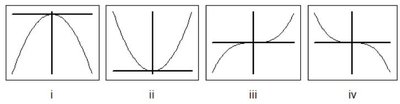
Appendix: Table Interpretation Example

Image	Description
i	Negative leading coefficient (opens downward)
ii	Positive leading coefficient (opens upward)
iii	Positive leading coefficient (rises to the right)
iv	Negative leading coefficient (falls to the right)