Calculus Study Guide: Limits and Continuity (Chapter 2)

Section 2.1 – The Idea of Limits

Review of Slope and Lines

Calculus begins with concepts from algebra, such as finding the slope and equation of a line. These ideas are foundational for understanding limits, average velocity, and the slope of tangent lines.

• Slope Formula: The slope m between two points $(x_1, y_1)$ and $(x_2, y_2)$ is given by: $m = \frac{y_2 - y_1}{x_2 - x_1}$

• Equation of a Line: The point-slope form is: $y = m(x - x_1) + y_1$

• Example: For points (2, 4) and (4, 16): $m = \frac{16 - 4}{4 - 2} = 6$ Equation: $y = 6(x - 2) + 4$

Introduction to Limits

A limit describes the value that the outputs of a function approach as the inputs approach a given value. This concept is central to calculus, especially in defining instantaneous velocity and the slope of a tangent line.

• Limit Notation: $\lim_{x \to a} f(x)$

• Secant Line: A line passing through two points on a graph; its slope represents average velocity.

• Tangent Line: A line touching the graph at one point; its slope represents instantaneous velocity.

Average and Instantaneous Velocity

Average velocity is calculated over an interval, while instantaneous velocity is the limit as the interval shrinks to a single point.

• Average Velocity Formula: $v_{av} = \frac{s(t_1) - s(t_0)}{t_1 - t_0}$

• Instantaneous Velocity: The limit of average velocity as $t_1 \to t_0$: $v_{inst} = \lim_{t_1 \to t_0} \frac{s(t_1) - s(t_0)}{t_1 - t_0}$

• Example: Using a table of positions, as the interval shrinks, the average velocity approaches the instantaneous velocity.

Section 2.2 – Definition of Limits

Informal and One-Sided Limits

Limits can be approached from the left or right. The notation distinguishes these cases:

• Right-Sided Limit: $\lim_{x \to a^+} f(x) = L$

• Left-Sided Limit: $\lim_{x \to a^-} f(x) = L$

• Limit of a Function: $\lim_{x \to a} f(x) = L$ if $f(x)$ approaches $L$ as $x$ approaches $a$ (but $x \neq a$).

• Existence of Limit: The limit exists if both one-sided limits are equal.

Examples Using Graphs and Tables

• Piecewise Functions: Limits may differ from the function value at a point.

• Example: For $f(x) = \frac{x^2 - 4}{x - 2}$, $f(2)$ is undefined, but $\lim_{x \to 2} f(x) = 4$.

Section 2.3 – Techniques for Computing Limits

Limit Laws and Theorems

Several laws simplify the computation of limits for sums, differences, products, quotients, powers, and roots.

• Sum Law: $\lim_{x \to a} [f(x) + g(x)] = \lim_{x \to a} f(x) + \lim_{x \to a} g(x)$

• Difference Law: $\lim_{x \to a} [f(x) - g(x)] = \lim_{x \to a} f(x) - \lim_{x \to a} g(x)$

• Product Law: $\lim_{x \to a} [f(x) \cdot g(x)] = \lim_{x \to a} f(x) \cdot \lim_{x \to a} g(x)$

• Quotient Law: $\lim_{x \to a} \frac{f(x)}{g(x)} = \frac{\lim_{x \to a} f(x)}{\lim_{x \to a} g(x)}$ (if denominator limit is not zero)

• Power Law: $\lim_{x \to a} [f(x)]^n = [\lim_{x \to a} f(x)]^n$

• Root Law: $\lim_{x \to a} \sqrt[n]{f(x)} = \sqrt[n]{\lim_{x \to a} f(x)}$ (if $f(x) > 0$ for even $n$)

Limits of Polynomial and Rational Functions

• Polynomial: $\lim_{x \to a} p(x) = p(a)$

• Rational: $\lim_{x \to a} \frac{p(x)}{q(x)} = \frac{p(a)}{q(a)}$ (if $q(a) \neq 0$)

Squeeze Theorem

The Squeeze Theorem helps find limits when a function is bounded between two others with the same limit.

• Theorem: If $f(x) \leq g(x) \leq h(x)$ near $a$ and $\lim_{x \to a} f(x) = \lim_{x \to a} h(x) = L$, then $\lim_{x \to a} g(x) = L$.

• Example: $\lim_{x \to 0} x^2 \cos x = 0$ by bounding $x^2 \cos x$ between $-x^2$ and $x^2$.

• 

Trigonometric Limits

• Example: $\lim_{x \to 0} \frac{\sin 2x}{x} = 2$

• Indeterminate Forms: Direct substitution may fail; use identities or algebraic manipulation.

Section 2.4 and 2.5 – Limits Involving Infinity

Infinite Limits and Limits at Infinity

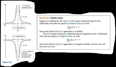
Limits involving infinity occur when function values grow without bound or when the input variable approaches infinity.

• Infinite Limit: $\lim_{x \to a} f(x) = \infty$ or $-\infty$ if $f(x)$ grows arbitrarily large as $x$ approaches $a$.

• 

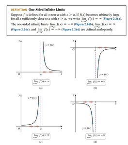
• One-Sided Infinite Limits: $\lim_{x \to a^+} f(x) = \infty$ or $-\infty$; $\lim_{x \to a^-} f(x) = \infty$ or $-\infty$.

• 

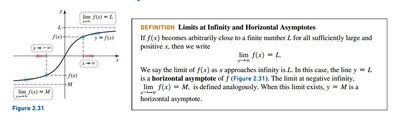
• Limit at Infinity: $\lim_{x \to \infty} f(x) = L$ if $f(x)$ approaches a finite value $L$ as $x$ grows large.

• 

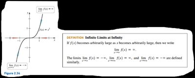
• Infinite Limits at Infinity: $\lim_{x \to \infty} f(x) = \infty$ or $-\infty$ if $f(x)$ grows without bound as $x$ increases.

• 

Vertical and Horizontal Asymptotes

• Vertical Asymptote (VA): Occurs where the denominator of a rational function is zero and the function grows without bound.

• Horizontal Asymptote (HA): Occurs when $f(x)$ approaches a finite value as $x$ approaches infinity.

• Degree Comparison:

  • If degree of numerator > degree of denominator: No HA

  • If degrees are equal: HA is ratio of leading coefficients

  • If degree of numerator < degree of denominator: HA is $y = 0$

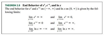
End Behavior of Exponential and Logarithmic Functions

• Theorem 2.8: End behavior for $e^x$, $e^{-x}$, and $\ln x$:

Function	$x \to \infty$	$x \to -\infty$
$e^x$	$\infty$	$0$
$e^{-x}$	$0$	$\infty$
$\ln x$	$\infty$	$-\infty$

• 

Section 2.6 – Continuity

Definition and Checklist for Continuity

A function is continuous at a point if its graph has no holes, jumps, or breaks. Most familiar functions are continuous everywhere, but some have points of discontinuity.

• Continuity Checklist:

  1. $f(a)$ is defined (a is in the domain).

  2. $\lim_{x \to a} f(x)$ exists.

  3. $\lim_{x \to a} f(x) = f(a)$

• Point of Discontinuity: Where the function fails to be continuous.

Types of Functions and Continuity

• Polynomial Functions: Continuous everywhere.

• Rational Functions: Continuous where denominator is not zero.

• Composite Functions: If $g$ is continuous at $a$ and $f$ is continuous at $g(a)$, then $f \circ g$ is continuous at $a$.

• Root Functions: If $n$ is odd, $\sqrt[n]{f(x)}$ is continuous wherever $f(x)$ is continuous. If $n$ is even, $\sqrt[n]{f(x)}$ is continuous where $f(x) > 0$.

• Inverse Functions: If $f$ is continuous and invertible on an interval, $f^{-1}$ is also continuous on the image of that interval.

Continuity at Endpoints and on Intervals

• Right-Continuous: $\lim_{x \to a^+} f(x) = f(a)$

• Left-Continuous: $\lim_{x \to a^-} f(x) = f(a)$

• Continuous on Interval: Continuous at every point in the interval; at endpoints, continuous from the appropriate side.

Intermediate Value Theorem (IVT)

The IVT states that if $f$ is continuous on $[a, b]$ and $L$ is between $f(a)$ and $f(b)$, then there exists $c$ in $(a, b)$ such that $f(c) = L$. This theorem guarantees the existence of a value but not its exact location.

• Application: Used to show that a solution exists for equations involving continuous functions.

• Example: If you invest $1000$and want $1300$ after 5 years, IVT guarantees an interest rate between $0 ext{%}$ and $8 ext{%}$ will achieve this.