Calculus Study Notes: Limits, Continuity, Differentiation, and Applications

Limits

Understanding Limits

Limits are foundational to calculus, describing the behavior of functions as the input approaches a particular value. They help us understand instantaneous rates of change and the continuity of functions.

• Definition: The limit of a function f(x) as x approaches a value a is L, written as $\lim_{x \to a} f(x) = L$, if f(x) gets arbitrarily close to L as x approaches a.

• One-Sided Limits: The left-hand limit ($\lim_{x \to a^-} f(x)$) and right-hand limit ($\lim_{x \to a^+} f(x)$) must be equal and finite for the two-sided limit to exist.

• Infinite Limits and Vertical Asymptotes: If f(x) increases or decreases without bound as x approaches a, we write $\lim_{x \to a} f(x) = \infty$ or $-\infty$ and say x = a is a vertical asymptote.

Limit Laws

Limit laws allow us to evaluate limits algebraically, provided the individual limits exist:

• Sum/Difference Law: $\lim_{x \to a} [f(x) \pm g(x)] = \lim_{x \to a} f(x) \pm \lim_{x \to a} g(x)$

• Constant Multiple Law: $\lim_{x \to a} [c \cdot f(x)] = c \cdot \lim_{x \to a} f(x)$

• Product Law: $\lim_{x \to a} [f(x) \cdot g(x)] = \lim_{x \to a} f(x) \cdot \lim_{x \to a} g(x)$

• Quotient Law: $\lim_{x \to a} \frac{f(x)}{g(x)} = \frac{\lim_{x \to a} f(x)}{\lim_{x \to a} g(x)}$, if $\lim_{x \to a} g(x) \neq 0$

• Power Law: $\lim_{x \to a} [f(x)]^n = [\lim_{x \to a} f(x)]^n$

• Root Law: $\lim_{x \to a} \sqrt[n]{f(x)} = \sqrt[n]{\lim_{x \to a} f(x)}$

Indeterminate Forms

Expressions like $\frac{0}{0}$ are called indeterminate forms and require algebraic manipulation (factoring, conjugates, etc.) to resolve.

Limits at Infinity

As x approaches infinity, the behavior of polynomials and rational functions depends on the degrees of the numerator and denominator.

• Polynomials: The highest degree term dominates as $x \to \pm\infty$.

• Rational Functions: Compare degrees of numerator (m) and denominator (n):

  • m > n: Limit is $\pm\infty$

  • m < n: Limit is 0

  • m = n: Limit is the ratio of leading coefficients

Continuity

Definition of Continuity

A function f(x) is continuous at x = a if:

• f(a) is defined

• $\lim_{x \to a} f(x)$ exists

• $\lim_{x \to a} f(x) = f(a)$

If any condition fails, f(x) has a discontinuity at x = a.

Types of Discontinuities

Type	Condition
Removable	$\lim_{x \to a} f(x)$ exists, but $f(a)$ is not defined or not equal to the limit
Jump	$\lim_{x \to a^-} f(x) \neq \lim_{x \to a^+} f(x)$
Infinite	One or both one-sided limits are $\pm\infty$

The Intermediate Value Theorem (IVT)

If f(x) is continuous on [a, b] and z is between f(a) and f(b), then there exists c in [a, b] such that f(c) = z. This theorem guarantees the existence of roots within intervals where the function changes sign.

Differentiation

Average and Instantaneous Rate of Change

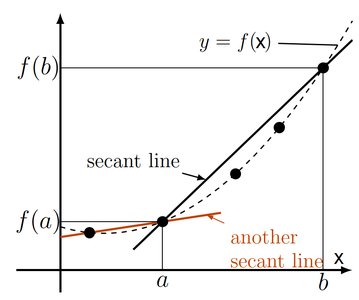
The average rate of change (AROC) of a function f(x) over [a, b] is the slope of the secant line:

• $\text{AROC} = \frac{f(b) - f(a)}{b - a}$

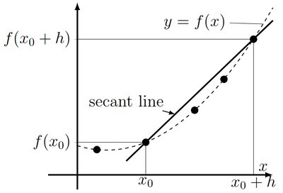
The instantaneous rate of change is the slope of the tangent line at a point, defined as the derivative:

• $f'(a) = \lim_{h \to 0} \frac{f(a + h) - f(a)}{h}$

The Derivative as a Function

The derivative function $f'(x)$ gives the instantaneous rate of change at any x:

• $f'(x) = \lim_{h \to 0} \frac{f(x + h) - f(x)}{h}$

Alternative notations: y', dy/dx, df/dx.

Rules of Differentiation

Rule	Formula
Constant	If $f(x) = c$, then $f'(x) = 0$
Constant Multiple	If $h(x) = c \cdot f(x)$, then $h'(x) = c \cdot f'(x)$
Sum/Difference	If $h(x) = f(x) \pm g(x)$, then $h'(x) = f'(x) \pm g'(x)$
Product	If $h(x) = f(x)g(x)$, then $h'(x) = f'(x)g(x) + f(x)g'(x)$
Quotient	If $h(x) = \frac{f(x)}{g(x)}$, then $h'(x) = \frac{f'(x)g(x) - f(x)g'(x)}{[g(x)]^2}$
Power	If $h(x) = x^n$, then $h'(x) = n x^{n-1}$

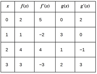
Using Tables for Derivatives

Given values of functions and their derivatives, you can compute derivatives of combinations using the rules above.

Higher Order Derivatives

The second derivative $f''(x)$ is the derivative of the derivative, representing the rate of change of the rate of change (e.g., acceleration if f(x) is position).

• Notation: $f''(x)$, $\frac{d^2y}{dx^2}$

Applications: Position, Velocity, and Acceleration

• Position: $s(t)$

• Velocity: $v(t) = s'(t)$

• Acceleration: $a(t) = v'(t) = s''(t)$

Related Rates and Implicit Differentiation

Related Rates

Related rates problems involve finding the rate at which one quantity changes by relating it to other quantities whose rates are known. The chain rule is essential:

• $\frac{dy}{dt} = \frac{dy}{dx} \cdot \frac{dx}{dt}$

Implicit Differentiation

For equations not solved for y, differentiate both sides with respect to x, treating y as a function of x and applying the chain rule when differentiating terms involving y.

Linearization and Differentials

Linear Approximation (Linearization)

The tangent line at x = a provides a linear approximation to f(x) near a:

• $L(x) = f(a) + f'(a)(x - a)$

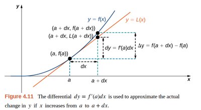
Differentials

The differential dy estimates the change in y for a small change dx in x:

• $dy = f'(a) dx$

Differential Equations and Growth Models

Exponential Growth and Decay

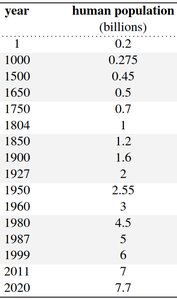
A differential equation relates a function to its derivatives. The simplest model for population growth is proportional growth:

• $\frac{dy}{dt} = ky$

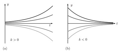
• General solution: $y = Ce^{kt}$

If k > 0, the solution represents exponential growth; if k < 0, exponential decay.

Initial Value Problems (IVP)

To find a specific solution, use an initial condition y(0) = y0:

• Solution: $y(t) = y_0 e^{kt}$

Applications

• Population dynamics, radioactive decay, pharmacokinetics, and more can be modeled using differential equations.

Additional info: This guide covers core calculus concepts including limits, continuity, differentiation, related rates, linearization, and introductory differential equations, with applications to life and social sciences. Images included are directly relevant to the explanation of the corresponding paragraphs.