Differential Equations: Methods, Applications, and Population Models

Differential Equations

Derivative Notation Systems

Differential equations use several notation systems to represent derivatives, each suited to different contexts and applications.

• Leibniz Notation: $\frac{dy}{dx}$, $\frac{d^2y}{dx^2}$ — Explicitly shows dependent and independent variables; ideal for separation of variables.

• Prime Notation: $y'$, $y''$, $y'''$ — Compact; used when the independent variable is obvious, often time.

• Dot Notation: $\dot{x}$, $\ddot{x}$ — Used almost exclusively for time derivatives; standard in mechanics and control theory.

• Operator Notation: $Dy = y'$, $D^2y = y''$ — Treats differentiation as an operator; useful in higher-order equations.

• Functional Notation: $y'(x)$, $y''(x)$, $f(x, y(x))$ — Emphasizes the function as a mapping; common in theoretical mathematics.

Definition and Order of Differential Equations

A differential equation contains an unknown function and its derivatives. The order of a differential equation is determined by the highest derivative present.

• General Solution: A family of functions that satisfy the equation.

• Initial Condition: Specifies a unique solution from the general family.

Solving Differential Equations

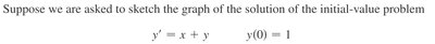
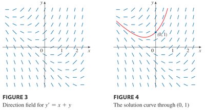
Direction Fields (Graphical Approach)

Direction fields provide a visual method for understanding the behavior of solutions to first-order differential equations. Each point in the plane is assigned a small line segment with slope equal to the value of the derivative at that point.

• Key Point: Direction fields help sketch solution curves without solving the equation analytically.

• Example: For the initial-value problem $y' = x + y$, $y(0) = 1$, the direction field and solution curve can be visualized.

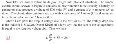
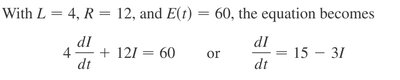
Physical Applications: Electric Circuits

Differential equations model physical systems such as electric circuits. For a circuit with resistance $R$, inductance $L$, and voltage $E(t)$, Kirchhoff's law gives:

• Equation: $L \frac{dI}{dt} + RI = E(t)$

• Application: Used to analyze current and voltage over time.

Equilibrium Solutions and Limiting Behavior

Direction fields can reveal equilibrium solutions and the long-term behavior of physical systems.

• Key Point: Solutions may approach a constant value as $t \to \infty$.

• Example: For $\frac{dI}{dt} = 15 - 3I$, all solutions approach $I = 5$.

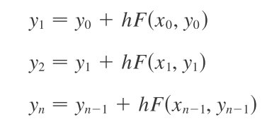
Numerical Methods: Euler's Method

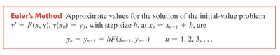
Euler's Method for Initial-Value Problems

Euler's Method is a numerical technique for approximating solutions to initial-value problems. It uses a step size $h$ to iteratively estimate values.

• Formula: $y_{n} = y_{n-1} + hF(x_{n-1}, y_{n-1})$

• Application: Useful when analytic solutions are difficult or impossible.

Example: Euler's Method Table

For $y' = x + y$, $y(0) = 1$, with $h = 0.1$:

• $y_1 = 1.1$

• $y_2 = 1.22$

• $y_3 = 1.362$

• ... (see table below)

n	x_n	y_n	n	x_n	y_n
1	0.1	1.100000	6	0.6	1.943122
2	0.2	1.220000	7	0.7	2.197434
3	0.3	1.362000	8	0.8	2.487178
4	0.4	1.528200	9	0.9	2.818595
5	0.5	1.721020	10	1.0	3.187485

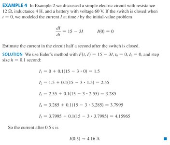
Example: Electric Circuit Current Estimation

Using Euler's Method for $\frac{dI}{dt} = 15 - 3I$, $I(0) = 0$, $h = 0.1$:

• $I_1 = 1.5$

• $I_2 = 2.55$

• $I_3 = 3.285$

• $I_4 = 3.7995$

• $I_5 = 4.15965$

So after 0.5 s, $I(0.5) \approx 4.16$ A.

Symbolic Methods: Separable and Linear Equations

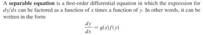
Separable Equations

A separable equation is a first-order differential equation where $\frac{dy}{dx}$ can be written as a product of a function of $x$ and a function of $y$:

• General Form: $\frac{dy}{dx} = g(x)f(y)$

• Solution Method: Separate variables and integrate both sides.

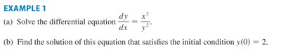
Example: Solving a Separable Equation

• Given $\frac{dy}{dx} = \frac{x^2}{y^2}$, separate and integrate:

• $y^2 dy = x^2 dx$

• Integrate: $\int y^2 dy = \int x^2 dx$

• Solution: $\frac{1}{3}y^3 = \frac{1}{3}x^3 + C$

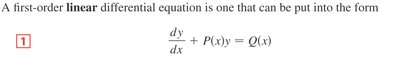
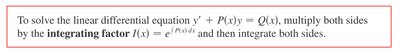
Linear First-Order Equations and Integrating Factor

A first-order linear differential equation can be written as:

• General Form: $\frac{dy}{dx} + P(x)y = Q(x)$

• Integrating Factor: $I(x) = e^{\int P(x)dx}$

• Solution Method: Multiply both sides by the integrating factor and integrate.

Example: Solving a Linear Equation

• Given $\frac{dy}{dx} + 3x^2y = 6x^2$

• Integrating factor: $e^{\int 3x^2 dx} = e^{x^3}$

• Solution: $y = 2 + Ce^{-x^3}$

Example: Electric Circuit with Integrating Factor

• Given $\frac{dI}{dt} + 3I = 15$, $I(0) = 0$

• Integrating factor: $e^{3t}$

• Solution: $I(t) = 5(1 - e^{-3t})$

Autonomous Equations

Definition

An autonomous equation is a differential equation where the independent variable does not appear explicitly on the right side:

• Form: $y' = f(y)$

Population Growth Models

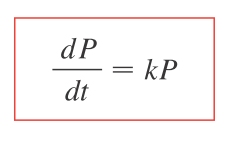
Law of Natural Growth

The law of natural growth models population growth as proportional to the current population:

• Equation: $\frac{dP}{dt} = kP$

• Solution: $P(t) = P_0 e^{kt}$

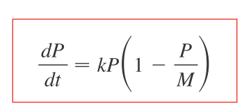
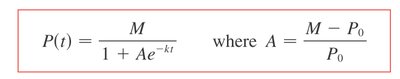
The Logistic Model

The logistic model incorporates a carrying capacity $M$, limiting population growth:

• Equation: $\frac{dP}{dt} = kP \left(1 - \frac{P}{M}\right)$

• Solution: $P(t) = \frac{M}{1 + Ae^{-kt}}$, where $A = \frac{M - P_0}{P_0}$

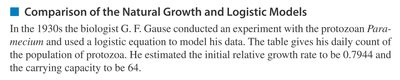
Comparison of Natural Growth and Logistic Models

Experiments, such as those by G. F. Gause with protozoa, demonstrate the logistic model's accuracy in predicting population growth with a carrying capacity.

• Key Point: Logistic models fit real-world population data better than natural growth models when resources are limited.

Summary of Key Concepts

• Differential Equation: Contains function and derivatives; used for modeling.

• Order: Highest derivative present.

• Direction Fields: Graphical approach to visualize solutions.

• Euler’s Method: Numerical approximation for initial-value problems.

• Separable Equations: Symbolic approach for certain first-order equations.

• Integration Factor: Symbolic approach for linear equations.

• Population Growth Models: Natural and logistic models for real-world applications.

Additional info: These notes expand on brief points with academic context, examples, and formulas to ensure completeness and clarity for calculus students.