Mathematical Models and Curve Fitting: Foundations for Calculus

Mathematical Models and Curve Fitting

Introduction to Mathematical Models

Mathematical models are equations or functions used to represent real-world data and phenomena. Curve fitting is the process of finding a mathematical model that best describes a set of data points, allowing predictions and analysis. This topic is foundational for calculus, as it introduces functions and their properties, which are essential for understanding limits, derivatives, and integrals.

Types of Functions Used in Curve Fitting

Several types of functions are commonly used to model data, each with distinct characteristics and applications:

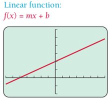
• Linear Function: Represents a straight-line relationship between variables. The general form is $f(x) = mx + b$, where m is the slope and b is the y-intercept.

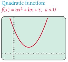
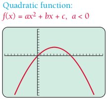
• Quadratic Function: Models data with a parabolic trend. The general form is $f(x) = ax^2 + bx + c$. If $a > 0$, the parabola opens upward; if $a < 0$, it opens downward.

• Polynomial Function: Extends beyond linear and quadratic, allowing for more complex curves. The general form is $f(x) = a_nx^n + \ldots + a_1x + a_0$.

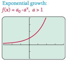
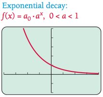
• Exponential Function: Used for rapid growth or decay. The general form is $f(x) = a_0 \cdot a^x$, with $a > 1$ for growth and $0 < a < 1$ for decay.

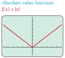
• Absolute-Value Function: Models V-shaped data, given by $f(x) = |x|$.

Identifying Appropriate Models from Data

To select a suitable model, examine the scatterplot or graph of the data:

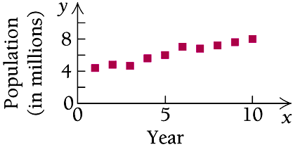
• Linear: Data points form a straight line.

• Quadratic: Data rises and falls in a parabolic shape.

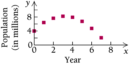
• Polynomial: Data rises and falls multiple times, not fitting linear or quadratic models.

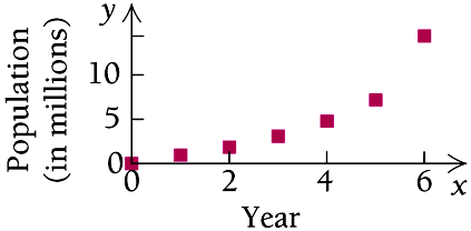
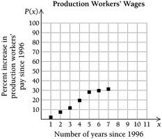
Example: Model Selection from Scatterplots

• Quadratic (a < 0): Data rises then falls in a curved manner.

• Linear: Data follows a straight line.

• Quadratic (a > 0): Data rises in a parabolic manner.

• Quadratic (a > 0): Data falls then rises in a curved manner.

• Polynomial: Data rises and falls more than once, indicating a higher-degree polynomial.

Curve Fitting: Linear Models

Linear models are used when data follows a straight-line trend. The process involves:

1. Plotting the data as a scatterplot.

2. Determining if the data fits a linear function.

3. Finding the linear equation by selecting two points and solving for m and b.

Example: For points (1, 1.9) and (4, 19.5):

• Set up equations: $1.9 = m \cdot 1 + b$, $19.5 = m \cdot 4 + b$

• Solve for $m$ and $b$:

• $m = \frac{19.5 - 1.9}{4 - 1} = 5.87$

• $b = 1.9 - 5.87 \cdot 1 = -3.97$

• Model: $P(x) = 5.87x - 3.97$

Prediction: For $x = 14$ (year 2010): $P(14) = 5.87 \cdot 14 - 3.97 = 78.21\%$

Curve Fitting: Quadratic Models

Quadratic models are used when data shows a parabolic trend. The process involves:

1. Plotting the data as a scatterplot.

2. Determining if the data fits a quadratic function.

3. Finding the quadratic equation by selecting three points and solving for a, b, and c.

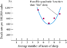
Example: For points (5, 1121), (7, 626), (9, 967):

• Set up equations: $y = ax^2 + bx + c$ for each point.

• Solve the system to find $a = 104.5$, $b = -1501.5$, $c = 601.6$

• Model: $y = 104.5x^2 - 1501.5x + 601.6$

Prediction:

• For $x = 2$: $y = 104.5 \cdot 2^2 - 1501.5 \cdot 2 + 601.6 = 3431$

• For $x = 8$: $y = 104.5 \cdot 8^2 - 1501.5 \cdot 8 + 601.6 = 692$

• For $x = 10$: $y = 104.5 \cdot 10^2 - 1501.5 \cdot 10 + 601.6 = 1451$

Quick Check: Fitting a Quadratic Model to Data

Given a table of data, use three points to fit a quadratic model and make predictions.

Age, x	Average Number of Live Births per 1000 women
16	34
18.5	86.5
22	111.1
27	113.9
32	84.5
37	35.4
42	6.8

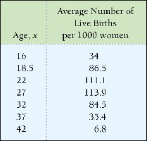
Example: Using points (16, 34), (22, 111.1), (32, 84.5):

• Set up equations: $y = ax^2 + bx + c$ for each point.

• Solve the system to find $a$, $b$, $c$.

• Model predicts 83.2 live births per 1000 women age 20.

Summary Table: Function Types and Their Applications

Function Type	General Form	Typical Application
Linear	$f(x) = mx + b$	Constant rate of change
Quadratic	$f(x) = ax^2 + bx + c$	Parabolic trends (rise/fall)
Polynomial	$f(x) = a_nx^n + \ldots + a_0$	Complex, multi-peak data
Exponential	$f(x) = a_0 \cdot a^x$	Growth/decay phenomena
Absolute Value	$f(x) = |x|$	V-shaped data

Conclusion: Understanding mathematical models and curve fitting is essential for analyzing data and making predictions. These concepts form the basis for more advanced calculus topics, including limits, derivatives, and integrals.