WTW 134 Calculus Study Guide – University of Pretoria

Theme 1 – Functions and Change

Unit 1.1: What is a Function?

A function is a rule that assigns to each element in a set (the domain) exactly one element in another set (the range). Understanding functions is foundational in calculus, as they model relationships between varying quantities.

• Domain: The set of all possible input values (x-values) for which the function is defined.

• Range: The set of all possible output values (y-values) the function can produce.

• Function Values: The output of a function for a given input, denoted as f(x).

• Intercepts: Vertical intercept is where the graph crosses the y-axis (set x = 0), and horizontal intercept is where it crosses the x-axis (set f(x) = 0).

• Increasing/Decreasing: A function is increasing on an interval if its values rise as x increases, and decreasing if its values fall.

• Concavity:

  • Concave up: All tangent lines lie below the graph on the interval.

  • Concave down: All tangent lines lie above the graph on the interval.

  • Linear functions are neither concave up nor down.

Example: For f(x) = x2, the function is increasing for x > 0, decreasing for x < 0, and concave up everywhere.

Unit 1.2: Types of Functions

There are several fundamental types of functions, each with characteristic formulas and graphs. Recognizing these types is essential for sketching and analyzing functions.

• Linear: $y = mx + b$

• Quadratic: $y = ax^2 + bx + c$

• Exponential: $y = a^x$

• Logarithmic: $y = \log_a(x)$ or $y = \ln(x)$

• Power: $y = x^n$

• Root: $y = \sqrt[n]{x}$

For each, the domain and range can be represented using interval notation.

Example: The function $y = e^{-x}$ is an exponential decay function with domain $(-\infty, \infty)$ and range $(0, \infty)$.

Unit 1.3: New Functions from Old Functions

Functions can be transformed by shifting, stretching, or reflecting their graphs. Composite functions are formed by applying one function to the result of another.

• Vertical shift: $y = f(x) + c$

• Horizontal shift: $y = f(x - c)$

• Vertical stretch/shrink: $y = cf(x)$

• Reflection about x-axis: $y = -f(x)$

• Reflection about y-axis: $y = f(-x)$

• Composite function: $h(x) = f(g(x))$

Example: If $f(x) = x^2$ and $g(x) = x + 1$, then $f(g(x)) = (x + 1)^2$.

Unit 1.4: Linear Functions

A linear function has the form $y = mx + b$, where $m$ is the slope (rate of change) and $b$ is the y-intercept. The symbol $\Delta$ denotes change (e.g., $\Delta x$ is the change in x).

• Equation of a line: $y - y_1 = m(x - x_1)$

• Recognizing linearity: If the rate of change between any two points is constant, the function is linear.

Example: For points (1,2) and (3,6), the slope is $m = (6-2)/(3-1) = 2$.

Unit 1.5: Rates of Change

The average rate of change of a function over an interval $[a, b]$ is the change in the function value divided by the change in x:

• $\text{Average rate of change} = \frac{f(b) - f(a)}{b - a}$

• Relative change: $\frac{f(b) - f(a)}{f(a)}$

• Velocity: If $s(t)$ is position, then average velocity over $[a, b]$ is $\frac{s(b) - s(a)}{b - a}$

Example: If $s(t) = t^2$, the average velocity from $t=1$ to $t=3$ is $\frac{9-1}{3-1} = 4$.

Unit 1.6: Continuity, Rate of Change, and the Derivative

A function is continuous on an interval if its graph has no breaks, holes, or jumps. The derivative at a point gives the instantaneous rate of change (the slope of the tangent line at that point).

• Estimating the derivative: Use average rates of change over small intervals near the point.

• Equation of tangent line: $y - f(a) = f'(a)(x - a)$

Example: For $f(x) = x^2$, at $x = 2$, $f'(2) = 4$, so the tangent line is $y - 4 = 4(x - 2)$.

Unit 1.7: The Derivative Function

The derivative function $f'(x)$ gives the rate of change of $f(x)$ at every point where it is defined. The sign of $f'(x)$ indicates whether $f(x)$ is increasing ($f'(x) > 0$), decreasing ($f'(x) < 0$), or constant ($f'(x) = 0$).

• If $f(x)$ is not continuous at $x = a$, then $f'(a)$ does not exist.

• If the graph has a corner at $x = a$, then $f'(a)$ does not exist.

Example: For $f(x) = |x|$, the derivative does not exist at $x = 0$ (corner point).

Theme 2 – Differentiation

Unit 2.1: Differentiation Formulas and Rules

Differentiation is the process of finding the derivative of a function. There are standard formulas and rules for differentiation:

• Power Rule: $\frac{d}{dx} x^n = n x^{n-1}$

• Constant Rule: $\frac{d}{dx} c = 0$

• Constant Multiple Rule: $\frac{d}{dx} [c f(x)] = c f'(x)$

• Sum Rule: $\frac{d}{dx} [f(x) + g(x)] = f'(x) + g'(x)$

• Product Rule: $\frac{d}{dx} [f(x)g(x)] = f'(x)g(x) + f(x)g'(x)$

• Quotient Rule: $\frac{d}{dx} \left[\frac{f(x)}{g(x)}\right] = \frac{f'(x)g(x) - f(x)g'(x)}{[g(x)]^2}$

• Chain Rule: $\frac{d}{dx} f(g(x)) = f'(g(x)) \cdot g'(x)$

Example: $\frac{d}{dx} (3x^2 + 2x) = 6x + 2$

Unit 2.2: The Chain Rule, Product Rule, and Quotient Rule

These rules are used to differentiate more complex functions:

• Chain Rule: For composite functions $y = f(g(x))$, $\frac{dy}{dx} = f'(g(x)) \cdot g'(x)$

• Product Rule: $\frac{d}{dx} [u(x)v(x)] = u'(x)v(x) + u(x)v'(x)$

• Quotient Rule: $\frac{d}{dx} \left[\frac{u(x)}{v(x)}\right] = \frac{u'(x)v(x) - u(x)v'(x)}{[v(x)]^2}$

Example: If $y = (2x + 1)^5$, then $y' = 5(2x + 1)^4 \cdot 2 = 10(2x + 1)^4$

Unit 2.3: Interpretations of the Derivative

The derivative can be interpreted as a rate of change, with units depending on the context (e.g., meters per second for velocity). The tangent line approximation uses the derivative to estimate function values near a point.

• Relative rate of change: $\frac{f'(x)}{f(x)}$

Example: If $f(x)$ is population at time $x$, then $f'(x)$ is the rate of population growth at time $x$.

Unit 2.4: The Second Derivative

The second derivative $f''(x)$ gives information about the concavity of a function:

• If $f''(x) > 0$, the function is concave up on that interval.

• If $f''(x) < 0$, the function is concave down on that interval.

Example: For $f(x) = x^3$, $f''(x) = 6x$, so the function is concave up for $x > 0$ and concave down for $x < 0$.

Theme 3 – Exponential, Logarithmic, Absolute Value, and Trigonometric Functions

Unit 3.1: Exponential Functions

An exponential function has the form $P = f(t) = a^t$, where $a > 0$. Exponential growth occurs when $a > 1$, and exponential decay when $0 < a < 1$.

• Growth/Decay Rate: Determined by the base $a$.

• Derivative: $\frac{d}{dt} a^t = a^t \ln a$

Example: $P = 2^t$ doubles as $t$ increases by 1.

Unit 3.2: Compound Interest and the Number e

Compound interest is calculated when interest is added to the principal at regular intervals. The number $e \approx 2.7183$ is the base for continuous compounding.

• Compound n times/year: $A = P\left(1 + \frac{r}{n}\right)^{nt}$

• Continuous compounding: $A = Pe^{rt}$

• Effective annual rate: $\left(1 + \frac{r}{n}\right)^n - 1$ or $e^r - 1$

Example: $1000 at 5\%$ compounded monthly for 1 year: $A = 1000\left(1 + \frac{0.05}{12}\right)^{12}$

Unit 3.3: The Natural Logarithm

The natural logarithm $\ln(x)$ is the inverse of the exponential function $e^x$. It is used to solve equations involving exponentials.

• Properties: $\ln(ab) = \ln a + \ln b$, $\ln(a^k) = k \ln a$, $e^{\ln x} = x$

• Domain: $x > 0$

Example: Solve $e^{2x} = 4 \implies 2x = \ln 4 \implies x = \frac{\ln 4}{2}$

Unit 3.4: Exponential Growth and Decay

Exponential growth and decay are modeled by $P = P_0 e^{kt}$, where $k > 0$ for growth and $k < 0$ for decay.

• Doubling time: $t = \frac{\ln 2}{k}$

• Half-life: $t = \frac{\ln 2}{|k|}$

Example: If $k = 0.1$, doubling time is $\frac{\ln 2}{0.1} \approx 6.93$ units.

Unit 3.5: Absolute Value Functions

The absolute value of $x$ is $|x| = x$ if $x \geq 0$, $-x$ if $x < 0$. The graph of $y = |f(x)|$ reflects the negative part of $f(x)$ above the x-axis.

• Solving equations: $|x| = a$ has solutions $x = a$ or $x = -a$.

• Solving inequalities: $|x| < a$ means $-a < x < a$.

Example: $|x - 2| = 3$ has solutions $x = 5$ or $x = -1$.

Unit 3.6: Periodic Functions

A periodic function repeats its values in regular intervals. The sine and cosine functions are periodic with period $2\pi$.

• General form: $y = A \sin(Bt) + C$ or $y = A \cos(Bt) + C$

• Amplitude: $|A|$

• Period: $\frac{2\pi}{|B|}$

Example: $y = 3 \sin(2t)$ has amplitude 3 and period $\pi$.

Theme 4 – Using the Derivative

Unit 4.1: Local Extremes of a Function

Local extremes are local maxima or minima. Critical points occur where $f'(x) = 0$ or $f'(x)$ is undefined. The First Derivative Test and Second Derivative Test are used to classify these points.

• First Derivative Test: Analyze sign changes of $f'(x)$ around critical points.

• Second Derivative Test: If $f''(c) > 0$, local minimum at $x = c$; if $f''(c) < 0$, local maximum.

Example: For $f(x) = x^2$, $f'(x) = 2x$, so $x = 0$ is a minimum.

Unit 4.2: Inflection Points

An inflection point is where the function changes concavity. It occurs where $f''(x) = 0$ and the sign of $f''(x)$ changes.

Example: For $f(x) = x^3$, $f''(x) = 6x$, so $x = 0$ is an inflection point.

Unit 4.3: Global Extremes of a Function

Global extremes are the highest or lowest values of a function on a given interval. For continuous functions on closed intervals, check endpoints and critical points.

• Evaluate $f(x)$ at all critical points and endpoints to find global maximum and minimum.

Example: For $f(x) = -x^2 + 4$ on $[-2, 2]$, maximum at $x = 0$, minimum at $x = -2$ and $x = 2$.

Theme 5 – Integration

Unit 5.1: Accumulated Change

Total change is visualized as the area under the graph of the rate of change function. Left-hand and right-hand sums estimate this area.

• Left-hand sum: Uses left endpoints of subintervals.

• Right-hand sum: Uses right endpoints of subintervals.

• Estimate: Average of left- and right-hand sums.

Unit 5.2: The Definite Integral

The definite integral $\int_a^b f(x) dx$ represents the net area under $f(x)$ from $x = a$ to $x = b$. The integrand is $f(x)$, and $a$, $b$ are the limits of integration.

• Estimate using tables, graphs, or formulas.

Unit 5.3: Antiderivatives

An antiderivative of $f(x)$ is a function $F(x)$ such that $F'(x) = f(x)$. The indefinite integral $\int f(x) dx$ represents all antiderivatives of $f(x)$.

• Basic integrals: $\int x^n dx = \frac{x^{n+1}}{n+1} + C$ (for $n \neq -1$)

• $\int e^x dx = e^x + C$

• $\int \sin x dx = -\cos x + C$

Unit 5.4: The Fundamental Theorem of Calculus

The Fundamental Theorem links differentiation and integration:

• If $F(x)$ is an antiderivative of $f(x)$, then $\int_a^b f(x) dx = F(b) - F(a)$

Theme 6 – Using the Definite Integral

Unit 6.1: The Definite Integral as Area

Definite integrals can be used to calculate the area between a function and the x-axis, or between two functions.

• Area between $y = f(x)$ and $y = g(x)$ from $x = a$ to $x = b$ is $\int_a^b |f(x) - g(x)| dx$

Unit 6.2: Interpretations of the Definite Integral

The definite integral can represent total change, with units determined by the context (e.g., total distance, total cost).

• Use the Fundamental Theorem to compute total change.

Unit 6.3: Average Value

The average value of a function $f(x)$ on $[a, b]$ is:

• $\text{Average value} = \frac{1}{b - a} \int_a^b f(x) dx$

Theme 7 – Function and Economics

Unit 7.1: Applications of Functions to Economics

Functions model economic quantities such as cost, revenue, profit, and depreciation.

• Cost function: $C(q)$, total cost for producing $q$ units.

• Revenue function: $R(q)$, total revenue from selling $q$ units.

• Profit function: $P(q) = R(q) - C(q)$

• Depreciation function: Value loss over time.

• Fixed costs: Costs that do not change with production level.

• Variable costs: Costs that change with production level.

• Supply and demand curves: Model the relationship between price and quantity supplied/demanded.

• Equilibrium: Where supply equals demand.

Unit 7.2: Marginal Cost and Revenue

Marginal cost is the derivative of the cost function, representing the cost of producing one more unit. Marginal revenue is the derivative of the revenue function.

• Marginal analysis uses derivatives to optimize profit, cost, or revenue.

Unit 7.3: Maximizing Profit, Cost, and Revenue

To maximize profit, cost, or revenue, set the derivative equal to zero and solve for the critical points. The relationship between marginal revenue and marginal cost determines the maximum profit point.

• Maximum profit occurs where marginal revenue equals marginal cost.

Unit 7.4: Finding Total Cost

Total cost can be found by integrating the marginal cost function and adding fixed costs. Similarly, total revenue is found by integrating the marginal revenue function.

Linear Algebra (Summary)

Unit 1.1: Matrix Addition and Scalar Multiplication

• Matrix: An $m \times n$ array of numbers.

• Matrix addition: Add corresponding entries.

• Scalar multiplication: Multiply every entry by the scalar.

Unit 1.2: Matrix Multiplication

• Product of $m \times n$ and $n \times r$ matrices is $m \times r$.

Unit 1.3: Systems of Linear Equations

• Use row operations to solve systems.

• Classify as consistent (unique or infinite solutions) or inconsistent (no solution).

Appendix: Visual Aids

The following image illustrates the sign of the leading term of polynomials based on their end behavior:

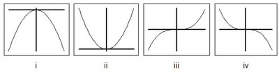
Explanation: The sign of the leading term determines the end behavior of the polynomial's graph. For example, if the leading coefficient is positive and the degree is even, both ends rise; if negative and even, both ends fall; if positive and odd, left falls and right rises; if negative and odd, left rises and right falls.