Analyzing Graphs of Polynomial Functions: Zeros, Extrema, and Modeling

Analyzing Graphs of Polynomial Functions

The Location Principle

The Location Principle is a method for approximating the zeros of a polynomial function by analyzing sign changes in function values. If a polynomial function f(x) changes sign between two consecutive values of x, then there is at least one real zero between those values.

• Definition: If f(a) < 0 and f(b) > 0 for real numbers a and b, then there is at least one real zero between a and b.

• Application: Construct a table of values for f(x) at consecutive integer values to locate intervals containing zeros.

• Example: For f(x) = x^4 - 2x^3 - x^2 + 1, a table of values reveals sign changes between x = 0 and x = 1, and between x = 2 and x = 3, indicating zeros in these intervals.

Note: Not all zeros can be found using the Location Principle, especially if the function does not change sign over an interval containing a zero.

Extrema of Polynomial Functions

Extrema are the relative maxima and minima of a function, also known as turning points. For a polynomial of degree n, there are at most n - 1 extrema.

• Relative Maximum: A point where the function changes from increasing to decreasing.

• Relative Minimum: A point where the function changes from decreasing to increasing.

• Finding Extrema: Use a table of values or a graphing calculator to estimate the x-coordinates of extrema.

• Example: For f(x) = x^3 + x^2 - 5x - 2, a table shows a maximum near x = -2 and a minimum near x = 1.

Key Features of Polynomial Graphs

When analyzing polynomial functions, it is important to describe their key features:

• Domain: The set of all possible input values (usually all real numbers for polynomials).

• Range: The set of all possible output values.

• Intercepts: Points where the graph crosses the axes (x-intercepts are zeros; y-intercept is f(0)).

• End Behavior: The behavior of the graph as x approaches positive or negative infinity, determined by the leading term.

• Symmetry: Even functions are symmetric about the y-axis; odd functions are symmetric about the origin.

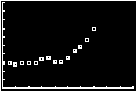
Modeling Data with Polynomial Functions

Polynomial functions can be used to model real-world data. The best-fitting polynomial can be found using regression techniques and graphing calculators.

• Scatter Plot: Plot the data points to visualize the trend.

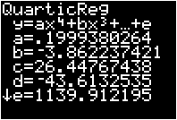
• Curve of Best Fit: Use regression (linear, quadratic, cubic, quartic) to find the polynomial that best fits the data. The best fit is indicated by the coefficient of determination (r^2) closest to 1.

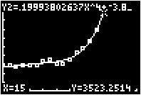
• Example: U.S. backpack sales data is modeled by a quartic regression equation:

$y \approx 0.2x^4 - 3.9x^3 + 26.4x^2 - 43.6x + 1139.9$

• To predict sales in 2015 (x = 15), substitute into the equation to get approximately $3,523$ million dollars.

Average Rate of Change

The average rate of change of a function over an interval [a, b] is given by:

$\text{Average Rate of Change} = \frac{f(b) - f(a)}{b - a}$

• Interpretation: This value represents the average change in the function's output per unit change in input over the interval.

• Example: For a rocket's acceleration, if $f(0) = 1.34$ Gs and $f(200) = 2.2$ Gs, the average rate of change is $(2.2 - 1.34)/200 = 0.0043$ Gs per second.

Practice and Application

• Use tables and graphs to locate zeros and extrema of polynomial functions.

• Model real-world data with polynomial regression and interpret the results.

• Calculate and interpret average rates of change in applied contexts.

Summary Table: Key Features of Polynomial Functions

Feature	Description	How to Find
Zeros (x-intercepts)	Values of x where f(x) = 0	Table, graph, or solve algebraically
Extrema	Relative maxima and minima (turning points)	Table, graph, or calculus (derivatives)
Intercepts	Where graph crosses axes	Set x = 0 for y-intercept; solve f(x) = 0 for x-intercepts
End Behavior	Graph's behavior as x → ±∞	Analyze leading term
Symmetry	Even: y-axis; Odd: origin	Test f(-x) = f(x) or f(-x) = -f(x)

Additional info: The images included above directly correspond to the process of modeling data with polynomial regression, as described in the "Modeling Data with Polynomial Functions" section. They show the scatter plot, regression coefficients, and the fitted curve with prediction, reinforcing the explanation of regression modeling.