College Algebra: Chapter 1 & 2 Study Notes

Review of Basic Algebra Skills

Order of Operations and Algebraic Manipulation

Understanding the foundational rules of algebra is essential for solving equations and simplifying expressions. The order of operations (PEMDAS/BODMAS) dictates the sequence in which calculations are performed: Parentheses/Brackets, Exponents/Orders, Multiplication and Division (from left to right), Addition and Subtraction (from left to right).

• Combining Like Terms: Add or subtract coefficients of terms with the same variable and exponent.

• Distributive Property: Multiply a single term across terms inside parentheses: $a(b + c) = ab + ac$.

• FOIL Method: Used for multiplying two binomials: $(a + b)(c + d) = ac + ad + bc + bd$.

Example: Simplify $(3x + 2) - (5x - 8)$: $3x + 2 - 5x + 8 = -2x + 10$.

Factoring

Common Factoring Techniques

Factoring is the process of expressing a polynomial as a product of its factors.

• Factoring out a Common Term: $ax + ay = a(x + y)$

• Difference of Squares: $A^2 - B^2 = (A + B)(A - B)$

• Factoring Trinomials: $x^2 + bx + c = (x + m)(x + n)$ where $m$ and $n$ are numbers that multiply to $c$ and add to $b$.

Example: Factor $x^2 - 49$: $x^2 - 49 = (x + 7)(x - 7)$.

Functions and Function Notation

Definition and Evaluation

A function is a relation where each input (independent variable, usually $x$) has exactly one output (dependent variable, usually $y$). Function notation is written as $y = f(x)$.

• Evaluating Functions: Substitute the input value into the function.

Example: If $f(x) = x^2 - 5x + 2$, then $f(2) = 2^2 - 5(2) + 2 = 4 - 10 + 2 = -4$.

Domain and Range

Definitions and Interval Notation

The domain of a function is the set of all possible input values (x-values). The range is the set of all possible output values (y-values). Intervals can be open $(a, b)$, closed $[a, b]$, or half-open $[a, b)$ or $(a, b]$.

• Closed Interval: $[a, b]$ includes endpoints.

• Open Interval: $(a, b)$ excludes endpoints.

Example: "Kayla got at least an 80 on the quiz, but no more than a 95" is $[80, 95]$.

Visualizing Functions

Graphical Interpretation

Graphs help visualize where a function is positive, negative, zero, increasing, decreasing, or constant.

• Positive Output: $f(x) > 0$ (above x-axis)

• Negative Output: $f(x) < 0$ (below x-axis)

• Zero Output: $f(x) = 0$ (x-intercepts)

• Increasing: $f(x)$ rises as $x$ increases

• Decreasing: $f(x)$ falls as $x$ increases

• Constant: $f(x)$ remains the same as $x$ increases

Average Rate of Change (Slope)

Definition and Calculation

The average rate of change of $y = f(x)$ between $x_1$ and $x_2$ is the slope of the line connecting the points $(x_1, y_1)$ and $(x_2, y_2)$:

$\text{Average Rate of Change} = \frac{y_2 - y_1}{x_2 - x_1}$

• Positive slope: output increases as input increases

• Negative slope: output decreases as input increases

• Zero slope: output is constant

Example: If LeBron scored 2,144 points in 2010 and 1,915 in 2022, the average rate of change is $(1915 - 2144)/(2022 - 2010) = -229/12 \approx -19.1$ points per year.

Linear Functions

General Form and Slope-Intercept Form

A linear function has a constant rate of change and its graph is a straight line. The general form is $y = mx + b$, where $m$ is the slope and $b$ is the y-intercept.

• Slope (m): Rate of change of $y$ with respect to $x$

• Y-intercept (b): Value of $y$ when $x = 0$

Example: For $12x - 2y = 4$, solve for $y$ to get $y = 6x - 2$ (slope $m = 6$, y-intercept $b = -2$).

Constructing Linear Graphs and Equations

Graphing and Writing Equations

• Plot the y-intercept ($b$)

• Use the slope ($m$) to find another point

• Connect the points to form a line

To write a linear equation from two points $(x_1, y_1)$ and $(x_2, y_2)$:

1. Find the slope: $m = \frac{y_2 - y_1}{x_2 - x_1}$

2. Plug one point and $m$ into $y = mx + b$ to solve for $b$

3. Write the equation in $y = mx + b$ form

Parallel and Perpendicular Lines

Relationships Between Slopes

• Parallel Lines: Same slope ($m_1 = m_2$)

• Perpendicular Lines: Slopes are negative reciprocals ($m_1 = -1/m_2$)

Linear Regression and Modeling Data

Fitting a Line to Data

When data does not perfectly fit a line, linear regression is used to find the best-fit line (regression line). This line minimizes the distance between the data points and the line itself.

• Calculator steps: Enter data, use LinReg function to find the equation $y = ax + b$

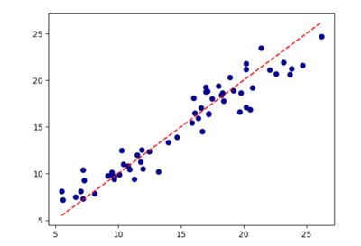
Example: The scatterplot above shows data points (blue dots) and the regression line (red dashed line) that best fits the data. The slope of the regression line represents the average rate of change between the variables.

Properties of Exponents

Exponent Rules

• Product Rule: $a^m a^n = a^{m+n}$

• Quotient Rule: $\frac{a^m}{a^n} = a^{m-n}$

• Power Rule: $(a^m)^n = a^{mn}$

• Product to Power: $(ab)^m = a^m b^m$

• Negative Exponent: $a^{-m} = \frac{1}{a^m}$

• Zero Exponent: $a^0 = 1$ (for $a \neq 0$)

Example: $(2m^2n^5)(4m^5n) = 8m^{2+5}n^{5+1} = 8m^7n^6$

Fractional Exponents and Radicals

Definitions and Simplification

• $a^{1/n} = \sqrt[n]{a}$

• $a^{m/n} = (\sqrt[n]{a})^m$

Example: $100^{1/2} = 10$; $x^{1/4} \cdot x^{3/4} = x^{(1/4)+(3/4)} = x^1 = x$

Logarithmic Functions

Definition and Properties

The logarithmic function with base $a$ is $y = \log_a x$ if and only if $x = a^y$. Common logarithms have base 10 ($\log x$), and natural logarithms have base $e$ ($\ln x$).

• $\log_a(a) = 1$

• $\log_a(1) = 0$

• $\log_a(a^x) = x$

• $a^{\log_a(x)} = x$

Change of Base Formula: $\log_a x = \frac{\ln x}{\ln a}$

Properties and Rules of Logarithms

• $\log_a(MN) = \log_a(M) + \log_a(N)$

• $\log_a\left(\frac{M}{N}\right) = \log_a(M) - \log_a(N)$

• $p \log_a(M) = \log_a(M^p)$

Example: $\log(25) + \log(2) = \log(50)$

Exponential Functions

Growth and Decay

An exponential function has the form $y = Ca^x$, where $C$ is the initial value and $a$ is the growth (if $a > 1$) or decay (if $0 < a < 1$) factor.

• Growth: $a = 1 + r$ where $r$ is the growth rate

• Decay: $a = 1 - r$ where $r$ is the decay rate

Example: If a population triples every period, $a = 3$; if it increases by 5% per year, $a = 1.05$.

Continuous Growth and Decay

Base $e$ Exponential Functions

The exponential function can also be written as $y = Pe^{rt}$, where $P$ is the initial amount and $r$ is the continuous growth or decay rate.

• If $r > 0$, the function models growth.

• If $r < 0$, the function models decay.

Example: $P(t) = 145e^{-0.092t}$ models a runner's pulse after a race.

Comparing Linear and Exponential Functions

Key Differences

• Linear Function: Constant difference between outputs; equation $y = mx + b$

• Exponential Function: Constant ratio between outputs; equation $y = Ca^x$

Example: If a club's membership increases by 10 people each year, it's linear; if it triples each year, it's exponential.