College Algebra Comprehensive Study Notes: Equations, Functions, Graphs, and Applications

Algebraic Equations

Solving Polynomial Equations

Polynomial equations are solved by factoring, completing the square, or using the quadratic formula. The solutions (roots) are the values of x that satisfy the equation.

• Factoring: Express the equation as a product of factors and set each factor to zero.

• Completing the Square: Rearrange the equation to form a perfect square trinomial.

• Quadratic Formula: For equations of the form $ax^2 + bx + c = 0$, use $x = \frac{-b \pm \sqrt{b^2 - 4ac}}{2a}$.

• Example: Solve $x^3 - 5x^2 = 7x - 35$ by factoring to get $(x-5)(x^2-7)=0$, so $x=5, \pm\sqrt{7}$.

Solving Radical and Rational Equations

Radical equations involve roots, and rational equations involve fractions. Isolate the radical or rational expression, then square or multiply both sides as needed, checking for extraneous solutions.

• Example: $\sqrt{m+7} - \sqrt{m-4} = 3$ leads to $m = \frac{37}{9}$ after isolating and squaring both sides.

Solving Absolute Value Equations and Inequalities

Absolute value equations are solved by considering both the positive and negative cases. For inequalities, express the solution in interval notation and graph on the real number line.

• Example: $|4x+2| - 11 = 15$ gives $x = 6$ or $x = -7$.

• Example (Inequality): $|x-5| + 3 < 15$ leads to $-7 < x < 17$.

Functions and Graphs

Definition and Identification of Functions

A function is a relation where each input (x) has exactly one output (y). Algebraically, solve for y and check if each x yields only one y.

• Example: $y = x^2 - 3$ is a function; $y = \pm\sqrt{x-3}$ is not a function.

Graphical Representation and Symmetry

Functions can be represented graphically. Symmetry can be tested algebraically or visually:

• y-axis symmetry: Replace x with -x; if unchanged, symmetric about y-axis.

• x-axis symmetry: Replace y with -y; if unchanged, symmetric about x-axis.

• Origin symmetry: Replace x with -x and y with -y; if unchanged, symmetric about the origin.

Type	Test	Example
y-axis	f(-x) = f(x)	y = x^2
x-axis	f(x) = -f(x)	Not a function
Origin	f(-x) = -f(x)	y = x^3

Common Functions and Their Graphs

Recognizing the shapes and properties of common functions is essential in algebra.

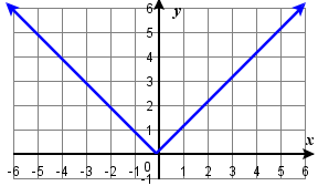
• Absolute Value: $f(x) = |x|$ is V-shaped, vertex at (0,0).

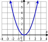
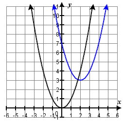
• Quadratic: $f(x) = x^2$ is U-shaped, vertex at (0,0).

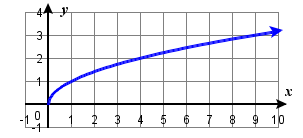
• Square Root: $f(x) = \sqrt{x}$ starts at (0,0), curves right.

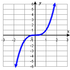
• Cubic: $f(x) = x^3$ is S-shaped, passes through (0,0).

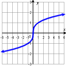
• Cube Root: $f(x) = \sqrt[3]{x}$ is a gentle S-curve through (0,0).

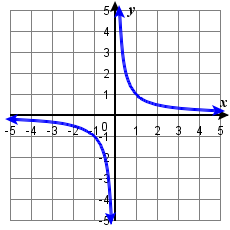
• Rational: $f(x) = \frac{1}{x}$ has two branches, asymptotes at x=0 and y=0.

Piecewise Functions

Piecewise functions are defined by different expressions over different intervals of the domain. Analyze each piece separately for domain, range, and intercepts.

• Example: $f(x) = \begin{cases} 2x-1 & x \leq 5 \\ x^2 & x > 5 \end{cases}$

Transformations of Functions

Functions can be shifted, reflected, stretched, or compressed. The order of transformations is important:

• Horizontal shift: $f(x-h)$ shifts right by h units.

• Vertical shift: $f(x) + k$ shifts up by k units.

• Reflection: $-f(x)$ reflects over x-axis; $f(-x)$ reflects over y-axis.

• Example: $a(x) = (x-2)^2 + 3$ is $y = x^2$ shifted right 2 and up 3.

Polynomial and Rational Functions

Quadratic Functions: Vertex, Axis of Symmetry, Intercepts

The standard form of a quadratic is $y = a(x-h)^2 + k$, where (h, k) is the vertex. The axis of symmetry is $x = h$.

• Vertex: $x = -\frac{b}{2a}$

• x-intercepts: Set $y=0$ and solve for $x$.

• y-intercept: Set $x=0$ and solve for $y$.

Finding Zeros and Factoring Polynomials

Zeros of a polynomial are the values of x where $f(x) = 0$. Use factoring, synthetic division, or the Rational Root Theorem to find zeros.

• Example: $f(x) = x^3 - 6x^2 + 5x + 12$ with known zero at $x=3$ can be factored using synthetic division.

Polynomial Division

Polynomials can be divided using long division or synthetic division. The Remainder Theorem states that the remainder of $f(x)$ divided by $(x-c)$ is $f(c)$.

• Example: $(2x^3 + 1) \div (x+1)$ using synthetic division.

End Behavior and Leading Coefficient Test

The end behavior of a polynomial function is determined by its degree and leading coefficient.

• Even degree, positive leading coefficient: Rises left and right.

• Odd degree, positive leading coefficient: Falls left, rises right.

• Even degree, negative leading coefficient: Falls left and right.

• Odd degree, negative leading coefficient: Rises left, falls right.

Exponential and Logarithmic Functions

Exponential Functions

Exponential functions have the form $y = a b^x$, where $b > 0$ and $b \neq 1$. The domain is $(-\infty, \infty)$ and the range is $(0, \infty)$ for $a > 0$.

• Horizontal asymptote: $y = 0$ (unless shifted).

• Inverse: The inverse of $y = b^x$ is $x = b^y$ or $y = \log_b x$.

Logarithmic Functions

Logarithmic functions are the inverses of exponential functions. The general form is $y = \log_b x$.

• Domain: $(0, \infty)$

• Range: $(-\infty, \infty)$

• Vertical asymptote: $x = 0$ (unless shifted).

Properties of Logarithms

• $\log_b (xy) = \log_b x + \log_b y$

• $\log_b \left(\frac{x}{y}\right) = \log_b x - \log_b y$

• $\log_b (x^k) = k \log_b x$

• $\log_b b = 1$

• $\log_b 1 = 0$

Solving Exponential and Logarithmic Equations

To solve exponential equations, take the logarithm of both sides. To solve logarithmic equations, rewrite in exponential form or use properties to combine logs.

• Example: $2^x = 8$ leads to $x = 3$.

• Example: $\log_2 (x-5) + \log_2 (x+2) = 3$ leads to $x^2 - 3x - 18 = 0$.

Applications

Variation Problems

Direct, inverse, and joint variation describe how one variable changes with respect to others.

• Direct variation: $y = kx$

• Inverse variation: $y = \frac{k}{x}$

• Joint variation: $y = kxz$

Exponential Growth and Decay

Exponential growth and decay are modeled by $A = A_0 e^{kt}$, where $k > 0$ for growth and $k < 0$ for decay.

• Half-life: The time required for a quantity to reduce to half its initial value.

• Doubling time: The time required for a quantity to double in size.

Compound Interest

Compound interest is calculated using $A = P \left(1 + \frac{r}{n}\right)^{nt}$, where $P$ is the principal, $r$ is the annual rate, $n$ is the number of compounding periods per year, and $t$ is the time in years.

Graphical Analysis and Interpretation

Interpreting Graphs of Functions

Understanding the key features of function graphs—such as intercepts, asymptotes, intervals of increase/decrease, and symmetry—is essential for analysis and applications.

• Intercepts: Points where the graph crosses the axes.

• Asymptotes: Lines the graph approaches but never touches.

• Intervals: Where the function is increasing, decreasing, positive, or negative.

Examples of Graphs and Their Properties

• Rational Function: $f(x) = \frac{1}{x}$ has vertical and horizontal asymptotes at $x=0$ and $y=0$ respectively.

• Quadratic Function: $f(x) = x^2$ is symmetric about the y-axis and has a vertex at (0,0).

• Absolute Value Function: $f(x) = |x|$ is V-shaped and symmetric about the y-axis.

• Ellipse: $x^2 + y^2 = r^2$ is symmetric about both axes.

• Sinusoidal Function: $f(x) = \sin(x)$ or $f(x) = \cos(x)$ is periodic and symmetric about the origin or y-axis depending on the function.

Summary Table: Common Functions and Their Properties

Function	Shape	Symmetry	Domain	Range
$f(x) = x^2$	U-shaped	y-axis	$(-\infty, \infty)$	$[0, \infty)$
$f(x) = |x|$	V-shaped	y-axis	$(-\infty, \infty)$	$[0, \infty)$
$f(x) = \sqrt{x}$	Curve right	None	$[0, \infty)$	$[0, \infty)$
$f(x) = x^3$	S-shaped	Origin	$(-\infty, \infty)$	$(-\infty, \infty)$
$f(x) = \frac{1}{x}$	Two branches	Origin	$(-\infty, 0) \cup (0, \infty)$	$(-\infty, 0) \cup (0, \infty)$