Exponential and Logarithmic Functions: Core Concepts and Applications

Chapter 4: Exponential and Logarithmic Functions

Exponential Rules

Understanding the rules of exponents is essential for manipulating exponential expressions and solving equations involving exponents. These rules are foundational for college algebra and are prerequisites for advanced topics.

• Product Rule: $a^n \cdot a^m = a^{n+m}$

• Product Rule (Different Bases): $a^n \cdot b^n = (a \cdot b)^n$

• Quotient Rule: $a^n \div a^m = a^{n-m}$

• Quotient Rule (Different Bases): $a^n \div b^n = \left(\frac{a}{b}\right)^n$

• Power Rule: $(b^n)^m = b^{n \cdot m}$

• Fractional Exponents: $b^{1/n} = \sqrt[n]{b}$

• General Rational Exponents: $b^{m/n} = (\sqrt[n]{b})^m$

• Negative Exponent Rule: $b^{-n} = \frac{1}{b^n}$

• Zero Exponent Rule: $b^0 = 1$

• One Exponent Rule: $b^1 = b$

• One to Any Power: $1^n = 1$

Example: Simplify $a^7 \cdot a^{-2} = a^{7+(-2)} = a^5$

Exponential Functions

Definition and Properties

An exponential function is defined as $f(x) = b^x$, where $b$ is a positive constant other than 1 ($b > 0$, $b \neq 1$), and $x$ is any real number. The base $b$ must be constant and positive.

• Examples: $f(x) = 2^x$, $f(x) = 3^{x+1}$, $f(x) = (1/4)^x$

• Non-examples: $f(x) = x^2$, $f(x) = x^x$, $f(x) = 1^x$ (variable base or base equals 1)

Exponential functions model many real-life phenomena, such as population growth, radioactive decay, and the spread of diseases.

Evaluating Exponential Functions

To evaluate an exponential function, substitute the given value of $x$ and compute the result. Calculators are often used for non-integer exponents.

• Example: $f(x) = 3.2 \cdot 4^x$ for $x = 5$

• Example: $h(x) = 7 \left(\frac{1}{2}\right)^x$ for $x = 6$

Graphing Exponential Functions

The graph of $f(x) = b^x$ depends on the value of $b$:

• If $b > 1$, the function is increasing.

• If $0 < b < 1$, the function is decreasing.

• The y-intercept is always at $(0, 1)$.

• There is no x-intercept.

• The horizontal asymptote is $y = 0$.

• The domain is $x \in (-\infty, \infty)$; the range is $y \in (0, \infty)$.

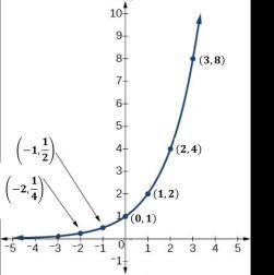
Example: The graph above shows $f(x) = 2^x$ passing through $(-2, 1/4)$, $(-1, 1/2)$, $(0, 1)$, $(1, 2)$, $(2, 4)$, and $(3, 8)$.

Comparing Exponential Growth and Decay

The value of $b$ determines the steepness of the graph:

• Larger $b$ values result in steeper increases (growth).

• Smaller $b$ values (between 0 and 1) result in steeper decreases (decay).

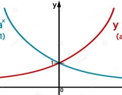
Example: $f(x) = 2^x$ (growth), $f(x) = (1/2)^x$ (decay).

The Number $e$

The mathematical constant $e$ is defined as the value that $\left(1 + \frac{1}{n}\right)^n$ approaches as $n$ becomes very large. It is approximately $e \approx 2.71828$.

• Exponential functions with base $e$: $f(x) = e^x$

• These functions are fundamental in calculus and continuous growth models.

Graph of $y = e^x$

The graph of $y = e^x$ shares the same general properties as other exponential functions with $b > 1$:

• Domain: $x \in (-\infty, \infty)$

• Range: $y \in (0, \infty)$

• Horizontal asymptote: $y = 0$

• Key points: $(0, 1)$, $(1, e)$, $(2, e^2)$

Applications: Compound Interest

Compound Interest Formula

Compound interest is calculated using the formula:

$A = P \left(1 + \frac{r}{n}\right)^{nt}$

• $A$ = final amount (future value)

• $P$ = initial principal (present value)

• $r$ = annual interest rate (as a decimal)

• $n$ = number of compounding periods per year

• $t$ = time in years

Compounding Period	n
Annually	1
Semiannually	2
Quarterly	4
Monthly	12
Weekly	52
Daily	365

Example: Amy deposits $10,000 at 9% annual interest, compounded monthly, for 5 years:

$A = 10,000 \left(1 + 0.0075\right)^{60} \approx 15,656.81$

Continuous Compound Interest

When interest is compounded continuously, the formula is:

$A = Pe^{rt}$

• $A$ = final amount

• $P$ = initial principal

• $r$ = annual interest rate (as a decimal)

• $t$ = time in years

Example: $2,340$ at 3.1% annual interest, compounded continuously for 3 years:

$A = 2340 \cdot e^{0.093} \approx 2,568.06$

Comparing Compounding Methods

To determine which investment method yields a higher return, compare the final amounts using both the compound interest and continuous compounding formulas.

• Example: Tony and Matt both invest $4,500 at 6% for 10 years. Tony's account is compounded quarterly, Matt's is compounded continuously. Calculate both final amounts and compare.

Summary Table: Key Properties of Exponential Functions

Property	Exponential Growth ($b > 1$)	Exponential Decay ($0 < b < 1$)
Domain	$(-\infty, \infty)$	$(-\infty, \infty)$
Range	$(0, \infty)$	$(0, \infty)$
y-intercept	$(0, 1)$	$(0, 1)$
Horizontal Asymptote	$y = 0$	$y = 0$
Behavior	Increasing	Decreasing