Exponential and Logarithmic Functions: Growth, Decay, and Modeling

Exponential Growth and Decay Models

Fundamental Concepts

Exponential functions are widely used to model situations where quantities grow or decay at rates proportional to their current value. These models are essential in fields such as biology, chemistry, economics, and population studies.

• Exponential Growth: Occurs when a quantity increases over time at a rate proportional to its current value.

• Exponential Decay: Occurs when a quantity decreases over time at a rate proportional to its current value.

• General Model: $f(t) = A_0 e^{kt}$ or $A = A_0 e^{kt}$, where:

  • $A_0$ is the initial amount

  • $k$ is the growth ($k > 0$) or decay ($k < 0$) rate

  • $t$ is time

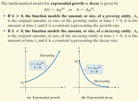
• Key Point: If $k > 0$, the function models growth; if $k < 0$, it models decay.

• Example: Population growth, radioactive decay, and financial investments.

Application Example: Population Growth

• Problem: In 2000, Africa's population was 807 million; by 2011, it was 1052 million. Find the exponential growth function and predict when the population will reach 2000 million.

• Solution: Use the exponential growth model $P(t) = P_0 e^{kt}$, where $P_0 = 807$ million and $t$ is years after 2000. Solve for $k$ using the 2011 data, then solve for $t$ when $P(t) = 2000$ million.

• Result: The population will reach 2000 million by the year 2038.

Application Example: Exponential Decay

• Problem: The half-life of strontium-90 is 28 years. Find the exponential decay model and determine how long it takes for 60 grams to decay to 10 grams.

• Solution: Use $A(t) = A_0 e^{kt}$, with $A_0 = 60$ grams. The decay constant $k$ is found using the half-life formula: $k = \frac{\ln(0.5)}{28}$.

• Result: It will take about 72 years for 60 grams to decay to 10 grams.

Logistic Growth Model

Limited Growth and Saturation

Logistic growth models describe situations where growth is limited by resources, leading to a saturation point. This is common in population dynamics and learning theory.

• General Model: $f(t) = \frac{c}{1 + a e^{-bt}}$, where:

  • $c$ is the limiting value (maximum possible size)

  • $a$ and $b$ are constants ($c > 0$, $b > 0$)

• Key Point: As $t \to \infty$, $f(t)$ approaches $c$.

• Example: Modeling the proportion of correct responses in learning trials.

Application Example: Learning Theory

• Problem: Psychologists use $f(t) = \frac{0.8}{1 + 1 e^{-0.2t}}$ to model correct responses after $t$ learning trials.

• Solution:

  • Prior to learning ($t = 0$): $f(0) = 0.4$

  • After 10 trials: $f(10) = 0.7$

  • Limiting value as $t \to \infty$: $f(t) \to 0.8$

Choosing an Appropriate Model for Data

Data Analysis and Model Selection

Selecting the right mathematical model for a set of data is crucial for accurate predictions and understanding relationships. Scatter plots help visualize the data and suggest suitable models.

• Example: Table 4.7 shows populations of cities and average walking speeds.

• Scatter Plot: Used to visualize the relationship between population and walking speed.

• Model Choice: The shape of the scatter plot suggests a logarithmic function is appropriate.

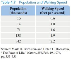
Population (thousands)	Walking Speed (feet per second)
5.5	0.6
14	1.0
71	1.6
138	1.9
342	2.2

Expressing Exponential Models in Base e

Conversion to Natural Exponential Form

Exponential models can be rewritten in terms of base $e$ for easier analysis and calculation, especially in calculus and advanced mathematics.

• General Conversion: $y = ab^x$ can be rewritten as $y = a e^{x \ln b}$.

• Example: Rewrite $y = 4(7.8)^x$ in terms of base $e$: $y = 4 e^{x \ln 7.8}$ Rounded to three decimal places: $y = 4 e^{2.054x}$

Summary

• Exponential and logarithmic functions are powerful tools for modeling growth, decay, and data relationships.

• Logistic models account for limited growth and saturation effects.

• Choosing the correct model for data is essential for accurate predictions.

• Expressing models in base $e$ simplifies calculations and analysis.