 Indietro
Predation and Predator-Prey Dynamics: Models and Responses
Guida di studio - Note intelligenti
 Appunti personalizzati basati sui tuoi materiali, ampliati con definizioni chiave, esempi e contesto.
Predation: Concepts and Types
Definition and Categories
Predation is a fundamental ecological interaction where one organism consumes another. Predators are heterotrophs that kill their prey immediately upon capture. Predation can be classified based on the type of tissue consumed:
Carnivores: Consume animal tissue.
Herbivores: Consume plant or algal tissue.
Omnivores: Consume both plant and animal tissue.
Cropping: Refers to partial consumption without killing the prey.
Lotka-Volterra Predator-Prey Model
Mathematical Formulation
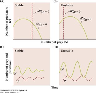
The Lotka-Volterra model describes the population dynamics of predator and prey species using differential equations. It assumes that predation is the only source of prey mortality and that predator birthrate is directly linked to prey consumption.
Prey Population Equation: Where r is the intrinsic rate of increase, c is the capture efficiency, N_{prey} is prey population size, and N_{pred} is predator population size.
Predator Population Equation: Where b is the birthrate per prey consumed, and d is the per capita death rate.
These equations link the two populations, each acting as a density-dependent regulator on the other.
Equilibrium Points
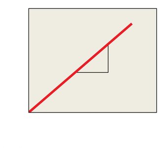
Prey Equilibrium: Occurs when
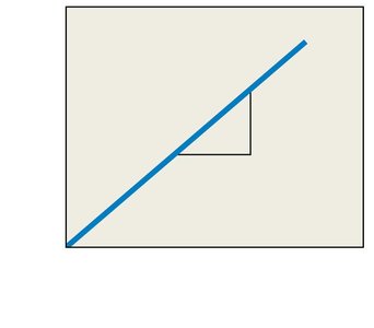
Predator Equilibrium: Occurs when
These points represent the population sizes at which growth rates are zero for each species.
Predator-Prey Dynamics
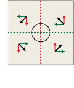
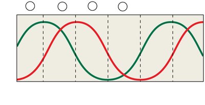
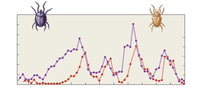
The predator population typically lags behind the prey population due to its dependence on prey availability. This results in oscillating population sizes over time.
Empirical Example: Mite Populations
An experiment with two mite species, Eotetranychus sexmaculatus (prey) and Typhlodromus occidentalis (predator), demonstrated oscillating population dynamics when environmental complexity allowed for refuges.
Predator Responses to Prey Density
Functional, Numerical, and Aggregative Responses
Functional Response: Change in the rate of prey consumption per predator as prey density changes.
Numerical Response: Change in predator population size due to reproduction, death, or migration in response to prey density.
Aggregative Response: Movement of predators into areas of high prey density.
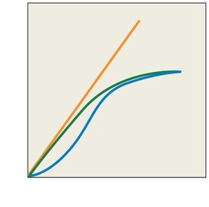
Types of Functional Responses
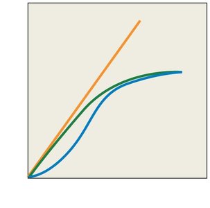
Functional responses describe how the number of prey consumed per predator per unit time changes with prey density:
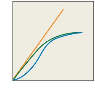
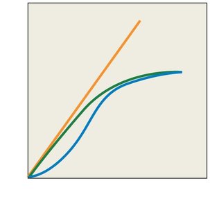
Type I: Linear increase in prey consumption with prey density; seen in passive predators like filter feeders.
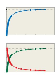
Type II: Decelerating increase due to handling time constraints; most common in nature.
Type III: Sigmoidal curve; low consumption at low prey density, then increases rapidly, then levels off.
Type I Functional Response
Assumes predators are never satiated and not limited by handling time. The proportion of prey consumed remains constant.
Type II Functional Response
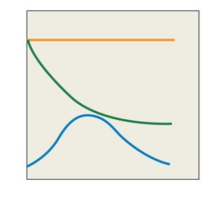
Includes handling time, leading to a maximum consumption rate at high prey density. The total feeding time (T) is divided into searching (Ts) and handling (Th).
Type III Functional Response
At low prey density, consumption rate is low due to limited search images and hiding spaces. As prey density increases, predators switch to more abundant prey, increasing mortality in a density-dependent manner.
Prey Switching and Search Image
Behavioral Adaptations
Predators may develop a search image for a particular prey, increasing their efficiency. When alternative prey becomes more abundant, predators may switch to the new prey species.
Prey Switching: Predators change their preference based on relative abundance and profitability of prey.
Numerical Responses and Population Regulation
Population Growth and Aggregation
Numerical responses can result from increased reproduction or immigration of predators into areas of high prey density. This response is crucial for regulating prey populations.
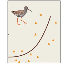
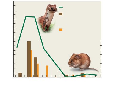
Field Example: Weasel and Rodent Populations
In a field study, weasel populations responded to rapid increases in rodent density, demonstrating a numerical response dominated by reproduction and aggregation.
Summary Table: Functional Response Types
Type | Shape | Key Features | Example |
|---|---|---|---|
Type I | Linear | Constant proportion consumed; no handling time | Filter feeders (e.g., plankton) |
Type II | Decelerating | Handling time limits consumption; most common | Most predators |
Type III | Sigmoidal | Low at low density, rapid increase, then plateau; prey switching | Predators with search image adaptation |
Key Equations
Prey population:
Predator population:
Equilibrium points: ,
Additional info: These notes expand on the brief points in the lecture slides, providing definitions, examples, and mathematical context for predator-prey dynamics and functional responses. Images included are directly relevant to the explanation of each paragraph, visually reinforcing key concepts.
