Confidence Intervals

Introduction to Confidence Intervals

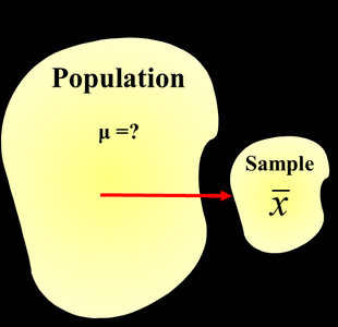
Confidence intervals are a fundamental concept in inferential statistics, allowing business analysts to estimate population parameters such as the mean or proportion based on sample data. A confidence interval provides a range of values, derived from a sample, that is likely to contain the true population parameter with a specified probability (confidence level).

• Point Estimate: A single value (e.g., sample mean) used as an estimate of a population parameter.

• Interval Estimate: A range of values within which the population parameter is expected to lie.

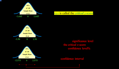
• Confidence Level: The probability that the interval estimate includes the population parameter (commonly 90%, 95%, or 99%).

• Margin of Error: The amount added and subtracted from the point estimate to form the confidence interval.

Theories Underlying Confidence Intervals

Two key statistical theories support the construction of confidence intervals:

• Empirical Rule: For a normal distribution, approximately 68% of values fall within ±1 standard deviation, 95% within ±2, and 99.7% within ±3.

• Central Limit Theorem (CLT): Regardless of the population distribution, the distribution of sample means approaches normality as sample size increases (n ≥ 30).

Critical Values and Confidence Levels

The critical value (zα/2 or tα/2) determines the width of the confidence interval. It is selected based on the desired confidence level and the distribution used (normal or t-distribution).

• zα/2: Used when population standard deviation is known and sample size is large.

• tα/2: Used when population standard deviation is unknown and sample size is small.

Calculating Confidence Intervals for the Mean (σ Known)

When the population standard deviation (σ) is known, the confidence interval for the mean is calculated using the normal distribution:

• Formula:

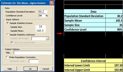
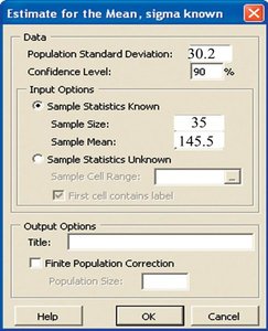
• Example: For a sample mean of 145.5, σ = 30.2, n = 35, and 90% confidence level (zα/2 = 1.645):

  • Standard error:

  • Interval: → [137.10, 153.90]

Finite Population Correction

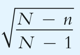
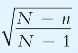
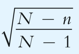
When sampling from a finite population (n/N > 0.05), a correction factor is applied to the standard error:

• Correction Factor:

• Adjusted Confidence Interval:

  • Upper Limit:

  • Lower Limit:

Calculating Confidence Intervals for the Mean (σ Unknown)

When the population standard deviation is unknown, the sample standard deviation (s) is used and the t-distribution is applied:

• Formula:

• Degrees of Freedom: df = n – 1

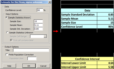
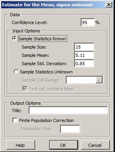
• Example: For a sample mean of 5.11, s = 0.85, n = 15, and 95% confidence level (tα/2 = 2.145):

  • Standard error:

  • Interval: → [4.64, 5.58]

Calculating Confidence Intervals for Proportions

Confidence intervals for proportions are used when estimating the probability of a success in a population. The binomial distribution is approximated by the normal distribution when np ≥ 5 and n(1 – p) ≥ 5.

• Formula:

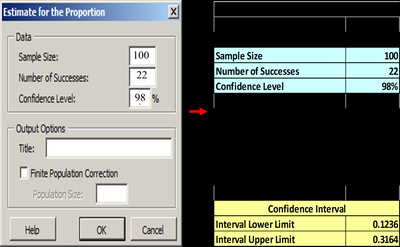
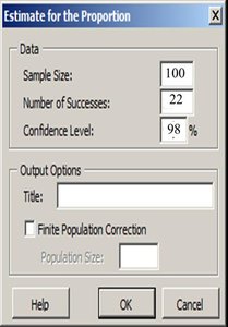
• Example: For 22 successes in 100 trials, 98% confidence level (zα/2 = 2.33):

  • Sample proportion:

  • Standard error:

  • Interval: → [0.124, 0.316]

Interpreting Confidence Intervals

It is important to interpret confidence intervals correctly:

• We are, for example, 95% confident that the true population parameter lies within the calculated interval.

• This does not mean there is a 95% probability that the interval contains the parameter; rather, 95% of intervals constructed from repeated samples will contain the parameter.

Summary Table: Types of Confidence Intervals

Applications in Business Statistics

• Estimating average sales, customer satisfaction, or defect rates.

• Validating claims (e.g., average battery life, fuel economy).

• Determining sample sizes for surveys and quality control.

Additional info: The notes above expand on the brief points in the slides, providing full academic context, definitions, and examples for each formula and concept. All images included directly reinforce the explanation of the adjacent paragraph, such as visualizing critical values, Excel calculations, and finite population corrections.