Applications of Integration

Overview

Integration is a fundamental tool in calculus with a wide range of applications. In this chapter, we focus on how integration is used to solve problems involving rates of change, such as velocity and acceleration, as well as geometric and physical applications like area, volume, and work. The central idea is that if the rate of change of a quantity is known, integration can be used to determine the net change or future value of that quantity over a given interval.

Velocity and Net Change

Position, Velocity, Displacement, and Distance

When an object moves along a straight line, its position at time t is denoted by s(t). The velocity v(t) is the rate of change of position, or the derivative of s(t). The displacement over a time interval [a, b] is the change in position, while the distance traveled is the total length of the path, regardless of direction.

• Position: is the location of the object relative to the origin at time .

• Velocity: is the rate of change of position.

• Displacement: is the net change in position over .

• Distance Traveled: is the total distance, always nonnegative.

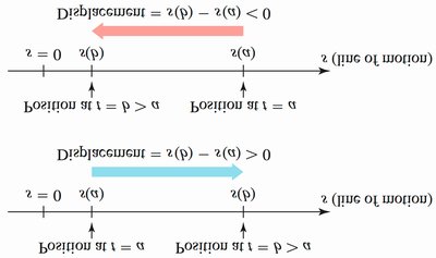
Key Point: Displacement can be positive or negative, depending on direction, while distance is always positive.

Graphical Interpretation

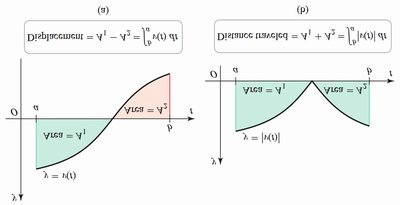
The definite integral of velocity over an interval gives the net area under the velocity curve, representing displacement. Integrating the speed (the absolute value of velocity) gives the total area under the curve, representing distance traveled.

Example: Jogger's Motion

Suppose a jogger's velocity is for (in mi/hr). To find displacement and distance:

• Find when to determine intervals of positive/negative motion.

• Compute and for displacement.

• Compute for distance (since is negative on ).

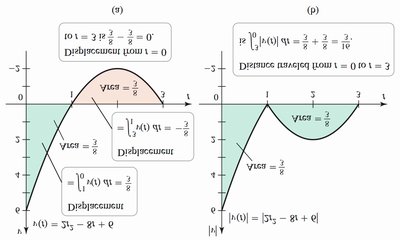
Example Calculation: Over , displacement is $0\frac{16}{3}$ mi.

Position from Velocity

If the velocity and initial position are known, the position at any time is:

This formula adds the initial position to the displacement over .

Example: Block on a Spring

A block is released from m with velocity . The position function is found by integrating the velocity and applying the initial condition:

The block oscillates, reaching the origin at , its highest point at , and repeats every seconds.

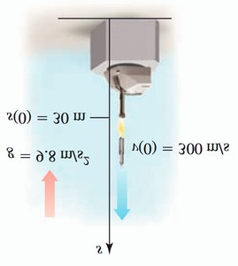
Velocity from Acceleration

Given acceleration and initial velocity , the velocity at time is:

This is analogous to finding position from velocity.

Net Change and Future Value

Generalization to Any Quantity

If a quantity changes at a known rate , then:

• Net Change:

• Future Value:

This applies to population, volume, cost, and more.

Example: Cell Growth

A cell culture starts with 100 cells and grows at a rate (cells/hr). The population at time is:

The population approaches 1000 as .

Example: Production Costs

If the marginal cost (rate of change of cost) is , the cost to produce from to units is:

Practice and Applications

Sample Problems

• Find displacement and distance for various velocity functions.

• Determine position from velocity using both antiderivatives and the Fundamental Theorem of Calculus.

• Apply integration to population growth, production, and physical scenarios like falling objects and energy consumption.

Graphical and Physical Applications

Integration is also used to compute:

• Area under curves (e.g., velocity-time, rate-time graphs)

• Volumes and surface areas of solids

• Work done by variable forces

• Total force exerted by fluids

Selected Graphs and Models

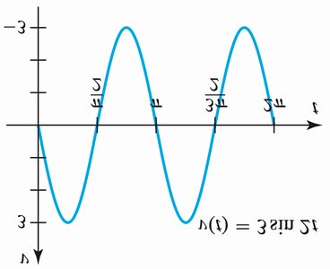
Example: The graph above shows a periodic velocity function, useful for calculating displacement and distance over intervals.

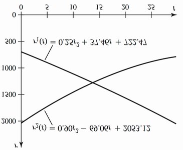
Example: Modeling river flow rates with quadratic functions to determine total water flow over a month.

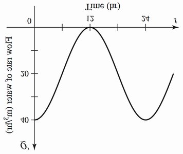
Example: Oscillating inflow rates require integration to find total volume added to a reservoir.

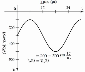
Example: Integrating power over time yields total energy consumption, important in engineering and environmental studies.

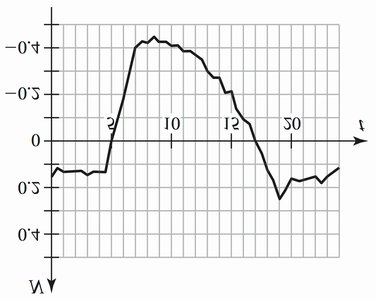
Example: The net ecosystem exchange graph shows periods of carbon uptake and release, with integration used to find total net change over a day.

Summary Table: Key Formulas

Additional info: These notes cover the foundational applications of integration in calculus, focusing on motion, accumulation, and physical modeling. The included images directly support the mathematical and conceptual explanations provided.