Chapter 1: Differentiation

Section 1.1: Limits – A Numerical and Graphical Approach

Limits are foundational to calculus, describing the behavior of functions as inputs approach specific values. Understanding limits is essential for defining derivatives and continuity.

• Definition of Limit: The limit of a function f(x) as x approaches a value a is the value that f(x) approaches as x gets arbitrarily close to a.

• Left-Hand and Right-Hand Limits: The left-hand limit (as x approaches a from the left) and the right-hand limit (as x approaches a from the right) must be equal for the overall limit to exist.

• Notation: (from the left), (from the right), (overall limit).

• Numerical Approach: Evaluate the function at values increasingly close to a from both sides.

• Graphical Approach: Observe the behavior of the graph as x approaches a.

Example: For the sequence 2.24, 2.249, 2.2499, ..., the numbers approach 2.25 from the left, so .

Theorem: if and only if both one-sided limits exist and are equal to L.

Non-Existence of Limits: If the left and right limits are not equal, the overall limit does not exist.

Graphical Illustration of Limits

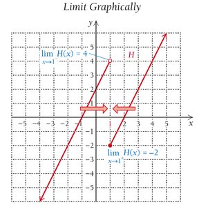
This graph shows how the left-hand and right-hand limits can differ, leading to the non-existence of the overall limit at a point.

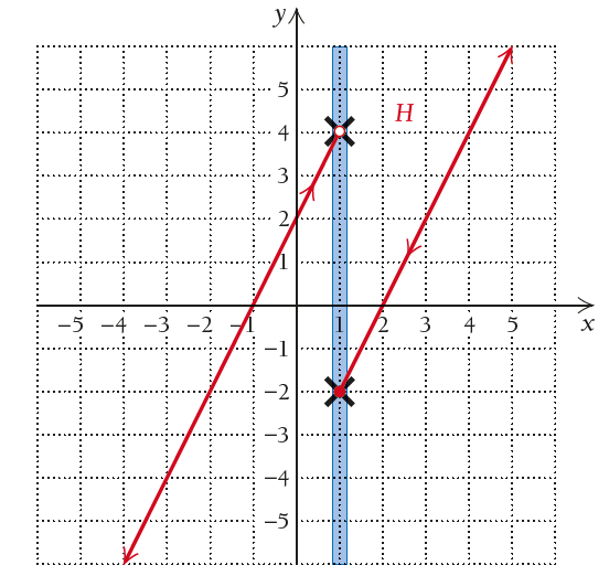
The "Wall" Method

The "wall" method visually demonstrates the process of approaching a point from both sides. If the values meet at the same point, the limit exists; otherwise, it does not.

Piecewise Functions and Limits

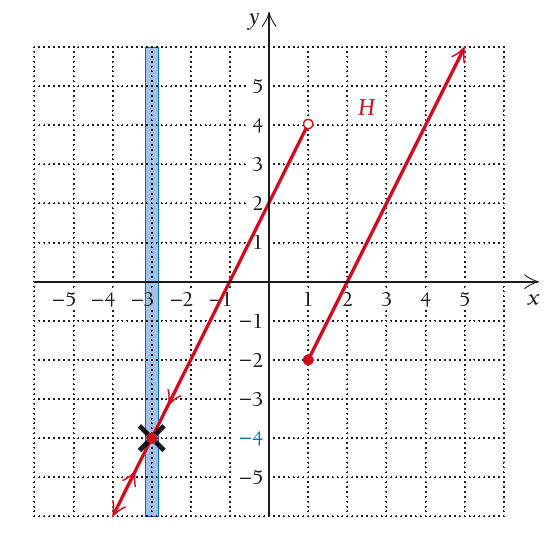
For piecewise functions, evaluate the limit from each side using the appropriate formula for each interval. If the values differ, the limit does not exist at that point.

Limits from Graphs

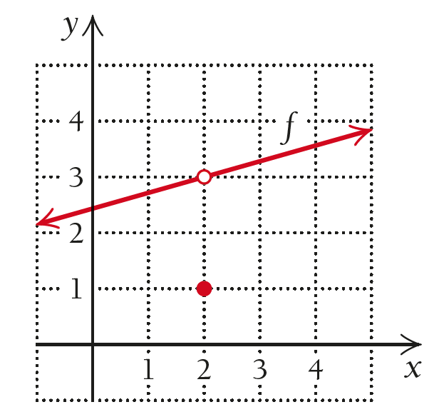
To find limits and function values from a graph, observe the y-value the function approaches as x nears the target value. If the function is not defined at that point, the limit may still exist.

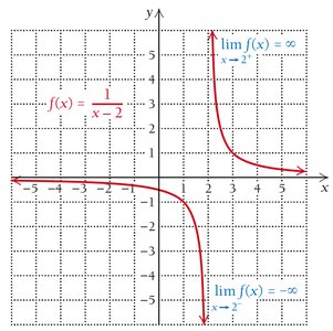
Infinite Limits

When a function increases or decreases without bound as x approaches a value, the limit is infinite or negative infinite. For example, as :

Section 1.2: Algebraic Limits and Continuity

This section introduces properties of limits and the concept of continuity, which are essential for differentiability.

• Limit Properties:

  • L1:

  • L2:

  • L3:

  • L4:

  • L5: , if denominator ≠ 0

  • L6:

• Continuity at a Point: A function f is continuous at if:

  1. f(a) exists

  2. exists

• Discontinuity: If any of the above conditions fail, f is discontinuous at x = a.

Section 1.3: Average Rates of Change

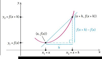
The average rate of change of a function over an interval measures how much the function's output changes per unit change in input.

• Formula:

• Units: The units are those of the output per unit of input (e.g., miles per hour).

• Difference Quotient: , where h ≠ 0, is the average rate of change over an interval of length h.

Section 1.4: Differentiation Using Limits of Difference Quotients

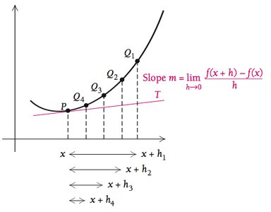
The derivative of a function at a point is the instantaneous rate of change, defined as the limit of the difference quotient as h approaches zero.

• Definition:

• Interpretation: The derivative represents the slope of the tangent line to the graph at x.

Differentiability

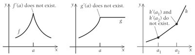
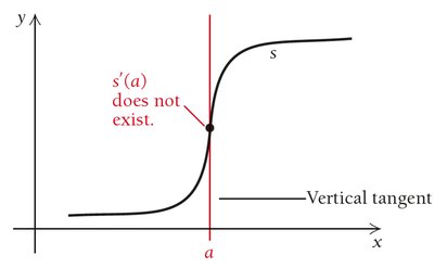
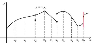
• A function is not differentiable at points where there is a corner, cusp, vertical tangent, or discontinuity.

Section 1.5: Leibniz Notation and the Power and Sum-Difference Rules

Leibniz notation expresses derivatives as , emphasizing the variables involved. The Power Rule and Sum-Difference Rule simplify differentiation of polynomials and sums/differences of functions.

• Power Rule: If , then

• Sum-Difference Rule: The derivative of a sum/difference is the sum/difference of the derivatives.

• Constant Multiple Rule: The derivative of a constant times a function is the constant times the derivative of the function.

Section 1.6: The Product and Quotient Rules

These rules allow differentiation of products and quotients of functions.

• Product Rule:

• Quotient Rule:

Section 1.7: The Chain Rule

The Chain Rule is used to differentiate composite functions.

• Chain Rule: If , then

• Extended Power Rule: For ,

Section 1.8: Higher-Order Derivatives

Higher-order derivatives are derivatives of derivatives. The second derivative measures the rate of change of the rate of change, and so on.

• Notation: or for the second derivative; or for the nth derivative.

• Applications: In physics, the first derivative of position is velocity, and the second derivative is acceleration.

Example: Velocity and Acceleration

• If is position, then is velocity, and is acceleration.

Summary Table: Differentiation Rules