Applications of Differentiation

Section 3.1: Using First Derivatives to Classify Maximum and Minimum Values and Sketch Graphs

This section introduces the use of the first derivative to determine where a function is increasing or decreasing, and to classify relative extrema (maximum and minimum points) of continuous functions. The First Derivative Test is a fundamental tool for analyzing the behavior of functions and sketching their graphs.

• Increasing Function: A function f is increasing on an interval I if for any a < b in I, f(a) < f(b).

• Decreasing Function: A function f is decreasing on I if for any a < b in I, f(a) > f(b).

• Theorem: If f'(x) > 0 for all x in I, then f is increasing on I. If f'(x) < 0, then f is decreasing on I.

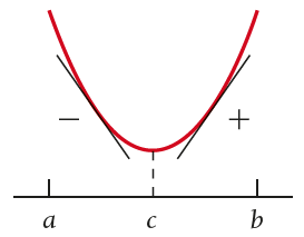
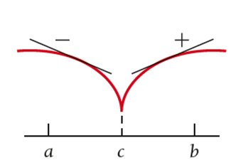
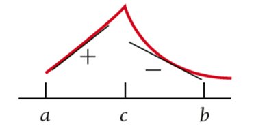
• Critical Value: A number c in the domain of f where f'(c) = 0 or f'(c) does not exist. The point (c, f(c)) is a critical point.

• First Derivative Test:

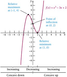
  • If f' changes from negative to positive at c, f has a relative minimum at c.

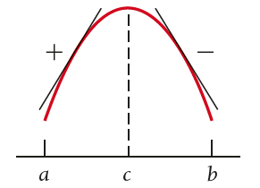
  • If f' changes from positive to negative at c, f has a relative maximum at c.

  • If f' does not change sign at c, there is no relative extremum at c.

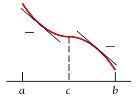
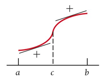
Example: Finding Relative Extrema

Given f(x) = (2/3)x^3 - 6x^2 + 12x, find the critical values by solving f'(x) = 2x^2 - 12x + 12 = 0. Analyze the sign of f'(x) in each interval to classify extrema using the First Derivative Test.

Section 3.2: Using Second Derivatives to Classify Maximum and Minimum Values and Sketch Graphs

The second derivative provides information about the concavity of a function and offers an alternative test for classifying relative extrema.

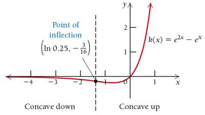
• Concave Up: f is concave up on I if f''(x) > 0 for all x in I.

• Concave Down: f is concave down on I if f''(x) < 0 for all x in I.

• Second Derivative Test: If f'(c) = 0 and f''(c) > 0, f has a relative minimum at c. If f''(c) < 0, f has a relative maximum at c. If f''(c) = 0, use the First Derivative Test.

• Point of Inflection: A point where f''(x) = 0 or f''(x) does not exist and the concavity changes.

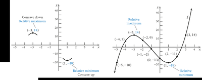
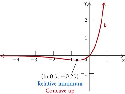
Section 3.3: Graph Sketching – Asymptotes and Rational Functions

This section covers the identification of vertical and horizontal asymptotes for rational, exponential, and logarithmic functions, and strategies for sketching their graphs.

• Rational Function: f(x) = P(x)/Q(x), where P and Q are polynomials and Q(x) ≠ 0.

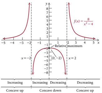
• Vertical Asymptote: The line x = a is a vertical asymptote if f(x) approaches infinity or negative infinity as x approaches a.

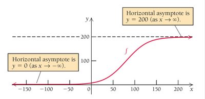
• Horizontal Asymptote: The line y = b is a horizontal asymptote if f(x) approaches b as x approaches infinity or negative infinity.

• Asymptotes for Exponential and Logarithmic Functions:

  • Exponential: y = 0 is a horizontal asymptote for f(x) = ae^{bx} as x → -∞ (if b > 0).

  • Logarithmic: x = a is a vertical asymptote for f(x) = \,ln(x-a).

Section 3.4: Optimization – Finding Absolute Maximum and Minimum Values

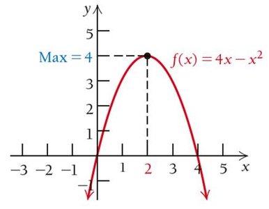
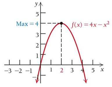
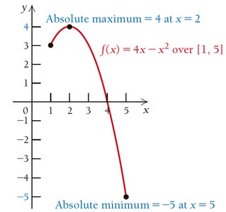
Optimization involves finding the largest or smallest value (absolute extrema) of a function on a given interval. The Extreme Value Theorem guarantees that a continuous function on a closed interval has both an absolute maximum and minimum.

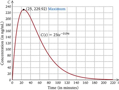
• Absolute Maximum: f(c) ≥ f(x) for all x in the domain.

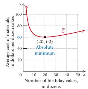
• Absolute Minimum: f(c) ≤ f(x) for all x in the domain.

• Extreme Value Theorem: A continuous function on [a, b] attains both an absolute maximum and minimum.

• Optimization Steps:

  1. Find f'(x).

  2. Find all critical values in [a, b].

  3. Evaluate f(x) at critical values and endpoints.

  4. The largest value is the absolute maximum; the smallest is the absolute minimum.

Section 3.5: Optimization – Business, Economic, and General Applications

Optimization techniques are widely used in business and economics to maximize profit, minimize cost, or optimize other quantities. The process involves translating a real-world problem into a mathematical model and applying calculus-based optimization methods.

• Strategy for Solving Maximum-Minimum Problems:

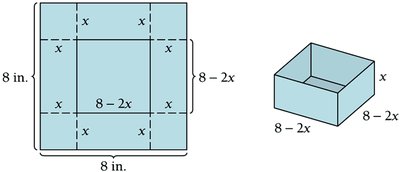
  1. Understand and diagram the problem.

  2. Define variables and constraints.

  3. Express the objective function in terms of one variable.

  4. Find critical points and use calculus to determine maxima or minima.

Section 3.6: Marginals, Differentials, and Linearization

This section introduces marginal analysis, differentials, and linearization, which are important for approximating changes and making local linear approximations of functions.

• Marginal Cost/Revenue/Profit: The derivative of the total cost/revenue/profit function, representing the approximate change for producing or selling one more unit.

• Differential: For y = f(x), the differential dy = f'(x)dx approximates the change in y for a small change dx in x.

• Linearization: The linear approximation of f(x) at x = a is L(x) = f(a) + f'(a)(x - a).

Section 3.7: Elasticity of Demand

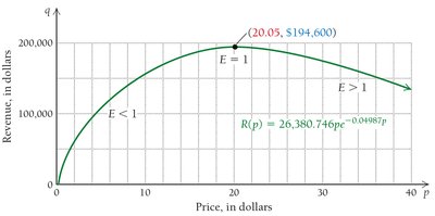
Elasticity of demand measures the responsiveness of quantity demanded to changes in price. It is a key concept in economics for maximizing revenue.

• Elasticity of Demand: E(p) = -p D'(p) / D(p), where D(p) is the demand function.

• Interpretation:

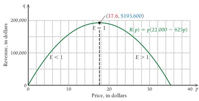
  • If E(p) < 1, demand is inelastic (revenue increases as price increases).

  • If E(p) > 1, demand is elastic (revenue decreases as price increases).

  • If E(p) = 1, revenue is maximized (unit elasticity).

Section 3.8: Implicit Differentiation and Logarithmic Differentiation

Implicit differentiation is used when functions are defined implicitly rather than explicitly. Logarithmic differentiation is useful for differentiating complicated products, quotients, or powers.

• Implicit Differentiation: Differentiate both sides of an equation with respect to x, treating y as a function of x.

• Logarithmic Differentiation: Take the natural logarithm of both sides before differentiating to simplify the process.

Section 3.9: Related Rates

Related rates problems involve finding the rate at which one quantity changes with respect to another, often time, when the quantities are related by an equation.

• Method:

  1. Write an equation relating the variables.

  2. Differentiate both sides with respect to time t.

  3. Substitute known values and solve for the desired rate.

Summary Table: Tests for Extrema and Concavity