Differential Equations: Methods, Applications, and Population Models

Guida di studio - Note intelligenti

Appunti personalizzati basati sui tuoi materiali, ampliati con definizioni chiave, esempi e contesto.

Differential Equations

Derivative Notation Systems

Differential equations use several notation systems to represent derivatives, each suited to different contexts and applications.

Leibniz Notation: , — Explicitly shows dependent and independent variables; ideal for separation of variables.
Prime Notation: , , — Compact; used when the independent variable is obvious, often time.
Dot Notation: , — Used almost exclusively for time derivatives; standard in mechanics and control theory.
Operator Notation: , — Treats differentiation as an operator; useful in higher-order equations.
Functional Notation: , , — Emphasizes the function as a mapping; common in theoretical mathematics.

Definition and Order of Differential Equations

A differential equation contains an unknown function and its derivatives. The order of a differential equation is determined by the highest derivative present.

General Solution: A family of functions that satisfy the equation.
Initial Condition: Specifies a unique solution from the general family.

Solving Differential Equations

Direction Fields (Graphical Approach)

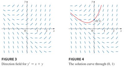
Direction fields provide a visual method for understanding the behavior of solutions to first-order differential equations. Each point in the plane is assigned a small line segment with slope equal to the value of the derivative at that point.

Key Point: Direction fields help sketch solution curves without solving the equation analytically.
Example: For the initial-value problem , , the direction field and solution curve can be visualized.

Direction field and solution curve for y' = x + y, y(0) = 1 Direction field for y' = x + y Solution curve through (0,1) for y' = x + y

Physical Applications: Electric Circuits

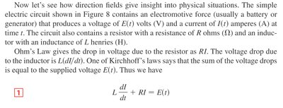
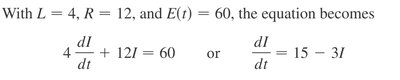
Differential equations model physical systems such as electric circuits. For a circuit with resistance , inductance , and voltage , Kirchhoff's law gives:

Equation:
Application: Used to analyze current and voltage over time.

Electric circuit differential equation

Equilibrium Solutions and Limiting Behavior

Direction fields can reveal equilibrium solutions and the long-term behavior of physical systems.

Key Point: Solutions may approach a constant value as .
Example: For , all solutions approach .

Numerical Methods: Euler's Method

Euler's Method for Initial-Value Problems

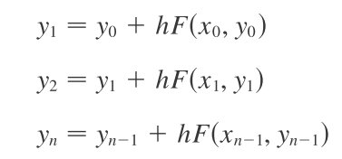
Euler's Method is a numerical technique for approximating solutions to initial-value problems. It uses a step size to iteratively estimate values.

Formula:
Application: Useful when analytic solutions are difficult or impossible.

Euler's Method formula Euler's Method explanation

Example: Euler's Method Table

For , , with :

... (see table below)

n	x_n	y_n	n	x_n	y_n
1	0.1	1.100000	6	0.6	1.943122
2	0.2	1.220000	7	0.7	2.197434
3	0.3	1.362000	8	0.8	2.487178
4	0.4	1.528200	9	0.9	2.818595
5	0.5	1.721020	10	1.0	3.187485

Euler's Method table of values

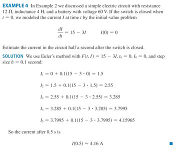
Example: Electric Circuit Current Estimation

Using Euler's Method for , , :

So after 0.5 s, A.

Euler's Method applied to electric circuit

Symbolic Methods: Separable and Linear Equations

Separable Equations

A separable equation is a first-order differential equation where can be written as a product of a function of and a function of :

General Form:
Solution Method: Separate variables and integrate both sides.

Separable equation form

Example: Solving a Separable Equation

Given , separate and integrate:
Integrate:
Solution:

Linear First-Order Equations and Integrating Factor

A first-order linear differential equation can be written as:

General Form:
Integrating Factor:
Solution Method: Multiply both sides by the integrating factor and integrate.

Integrating factor method

Example: Solving a Linear Equation

Given
Integrating factor:
Solution:

Linear equation solution example

Example: Electric Circuit with Integrating Factor

Given ,
Integrating factor:
Solution:

Electric circuit solution with integrating factor

Autonomous Equations

Definition

An autonomous equation is a differential equation where the independent variable does not appear explicitly on the right side:

Form:

Autonomous equation definition

Population Growth Models

Law of Natural Growth

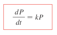
The law of natural growth models population growth as proportional to the current population:

Equation:
Solution:

Law of natural growth equation

The Logistic Model

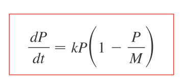
The logistic model incorporates a carrying capacity , limiting population growth:

Equation:
Solution: , where

Logistic model equation Logistic model solution

Comparison of Natural Growth and Logistic Models

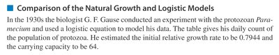
Experiments, such as those by G. F. Gause with protozoa, demonstrate the logistic model's accuracy in predicting population growth with a carrying capacity.

Key Point: Logistic models fit real-world population data better than natural growth models when resources are limited.

Comparison of growth models

Summary of Key Concepts

Differential Equation: Contains function and derivatives; used for modeling.
Order: Highest derivative present.
Direction Fields: Graphical approach to visualize solutions.
Euler’s Method: Numerical approximation for initial-value problems.
Separable Equations: Symbolic approach for certain first-order equations.
Integration Factor: Symbolic approach for linear equations.
Population Growth Models: Natural and logistic models for real-world applications.

Additional info: These notes expand on brief points with academic context, examples, and formulas to ensure completeness and clarity for calculus students.