Systems of Linear Equations

Introduction to Systems of Linear Equations

A system of linear equations consists of two or more linear equations considered simultaneously. The solution to the system is the set of variable values that satisfy all equations at once. For two variables, the solution corresponds to the intersection point of their graphs, if one exists.

• Consistent system: Has at least one solution.

• Inconsistent system: Has no solution (parallel lines).

• Dependent system: Has infinitely many solutions (coincident lines).

Example: Solve the system:

• y = 2x - 1

• y = -x + 8

Graphing Systems of Linear Equations

Graphing a Pair of Lines Together

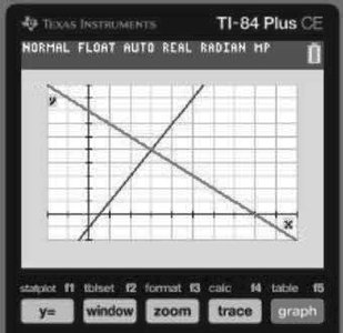
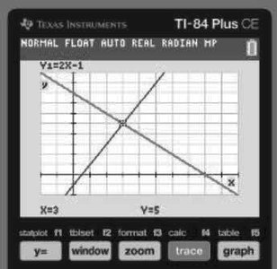
Graphing both equations on the same coordinate plane allows you to visually identify the intersection point, which is the solution to the system. This method is especially useful for systems with two variables.

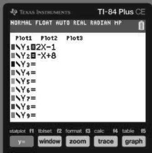
• Enter each equation into the calculator's Y= editor.

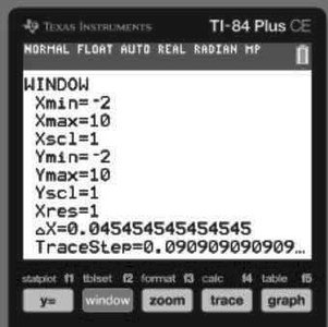
• Adjust the window to display the relevant portion of the graph.

• Use the graph and trace features to find the intersection point.

Algebraic Methods for Solving Systems

Solve by Substitution Method

The substitution method is effective when one equation is already solved for one variable. Substitute the expression for that variable into the other equation, solve for the remaining variable, and back-substitute to find the other value.

• Step 1: Solve one equation for one variable (if necessary).

• Step 2: Substitute this expression into the other equation.

• Step 3: Solve for the remaining variable.

• Step 4: Substitute back to find the other variable.

Example: Solve the system:

• y = x + 2

• y = 2x + 1

Set y = y: x + 2 = 2x + 1 → x = 1, then y = 1 + 2 = 3. Solution: (1, 3).

Solve by Elimination Method

The elimination method (also called the addition method) is useful for systems in standard form. Manipulate the equations so that adding or subtracting them eliminates one variable, allowing you to solve for the other.

• Step 1: Multiply one or both equations by a nonzero constant if necessary to align coefficients.

• Step 2: Add or subtract the equations to eliminate one variable.

• Step 3: Solve for the remaining variable.

• Step 4: Substitute back to find the other variable.

Example: Solve the system:

• x + 2y = 8

• x + y = 6

Subtract the second equation from the first: (x + 2y) - (x + y) = 8 - 6 → y = 2. Substitute into x + y = 6: x + 2 = 6 → x = 4. Solution: (4, 2).

Equation Manipulations

• Non-Zero Multiple: Multiplying an equation by a nonzero constant yields an equivalent equation.

• Add/Subtract Equations: Adding or subtracting equations produces another equivalent equation.

Applications of Systems of Linear Equations

Quantity-Value Systems

These systems involve two equations: one for the total quantity and one for the total value. Common in coin and mixture problems.

Example: Sonya has 30 coins (dimes and quarters) totaling $5.70. Let d = number of dimes, q = number of quarters.

• d + q = 30

• 0.10d + 0.25q = 5.70

Solve this system for d and q.

Break-Even Systems

Break-even analysis sets revenue equal to cost to determine the point at which a business neither makes nor loses money.

Example: It costs $10 per calculator to make the TI-84, with a monthly overhead of $24,500. Each calculator sells for $45. Let x = number of calculators.

• Cost: C = 10x + 24,500

• Revenue: R = 45x

Set R = C to find the break-even quantity: 45x = 10x + 24,500 → 35x = 24,500 → x = 700.

Large Systems of Linear Equations (3 or More Variables)

Systems in Three Variables

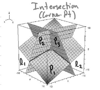
A linear equation in three variables (x, y, z) represents a plane in three-dimensional space. The intersection of two planes is a line; the intersection of three planes (if not parallel or coincident) is a single point.

Augmented Matrices and Row Operations

An augmented matrix is a rectangular array representing a system of equations, where each row corresponds to an equation and each column to a variable (plus one for constants). Row operations (multiplying by nonzero constants, adding/subtracting rows) are used to simplify the system, often to Reduced Row Echelon Form (RREF).

Example: System:

• x + 2y = 8

• x + y = 6

Augmented matrix:

Solving Systems with the TI-84 Calculator

The TI-84 calculator can be used to enter matrices and perform row operations, including finding the RREF to solve systems efficiently.

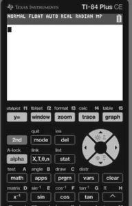
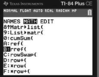
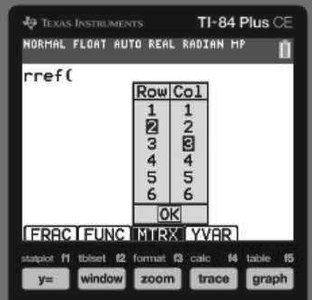
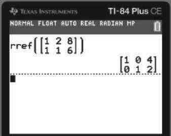
• Enter the augmented matrix using the [2nd] [MATRIX] menu.

• Select the rref( function to reduce the matrix.

• The resulting matrix gives the solution directly.

Example: For the system:

• x + 2y = 8

• x + y = 6

The calculator returns:

which means x = 4, y = 2.

Summary Table: Methods for Solving Systems

Key Formulas and Calculator Commands

• Slope-intercept form:

• Standard form:

• Break-even point:

• Augmented matrix:

• TI-84 RREF command: rref([matrix])