Expressing Solution Concentration

Overview of Concentration Units

Concentration describes the amount of solute present in a given quantity of solvent or solution. Several units are commonly used in chemistry to express concentration, each with specific applications and calculation methods.

• Mass Percent (%): The mass of solute divided by the total mass of solution, multiplied by 100.

• Parts Per Million (ppm): The mass of solute per million parts of solution mass.

• Parts Per Billion (ppb): The mass of solute per billion parts of solution mass.

• Molarity (M): Moles of solute per liter of solution.

• Molality (m): Moles of solute per kilogram of solvent.

• Mole Fraction (X): Moles of a component divided by the total moles of all components.

Key Equations:

• Mass Percent:

• ppm:

• ppb:

• Molarity:

• Molality:

• Mole Fraction:

Example: Lead in Drinking Water

The Environmental Protection Agency (EPA) sets a limit for lead in water at 15 ppb. To determine the maximum mass of lead allowed in 1.00 L of water (density = 1.00 g/cm3):

• Mass of solution = 1.00 L × 1000 mL/L × 1 g/mL = 1000 g

• Maximum mass of lead:

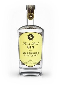
Example: Concentration Calculations for Ethanol in Gin

Given a gin solution labeled as 44% alcohol by volume, with the remainder water, and known densities, the following concentrations can be calculated for ethanol:

• Mass of ethanol (CH3CH2OH): 440 mL × 0.789 g/mL = 347 g

• Mass of water: 560 mL × 0.998 g/mL = 559 g

• Moles of ethanol:

• Moles of water:

• Mass percent ethanol:

• Mole fraction ethanol:

• Molarity:

• Molality:

Colligative Properties of Solutions

Definition and Overview

Colligative properties are physical properties of solutions that depend only on the number of solute particles present, not their identity. These properties arise due to the entropy-driven stabilization of the solution.

• Vapor Pressure Lowering

• Boiling Point Elevation

• Freezing Point Depression

• Osmotic Pressure

For ideal solutions, solvent–solute interactions are similar in strength to solute–solute and solvent–solvent interactions.

Vapor Pressure Lowering (Raoult’s Law)

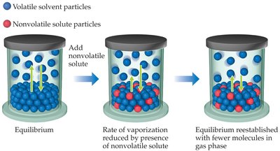
Adding a nonvolatile solute to a solvent lowers the solvent’s vapor pressure. This is described by Raoult’s Law:

• Where is the mole fraction of the solvent and is the vapor pressure of the pure solvent.

Example: Adding 22.5 g lactose (C12H22O11) to 100.0 g water at 25°C (vapor pressure of pure H2O = 23.8 torr):

• Moles lactose:

• Moles water:

• Mole fraction water:

• Vapor pressure of solution: torr

Ideal Solutions with Two Volatile Components

In solutions with two volatile components, each component contributes to the total vapor pressure according to Raoult’s Law. The total pressure is the sum of the partial pressures (Dalton’s Law):

Example: For gin (44% ethanol by volume), at 20°C, torr, torr, :

• torr

• torr

• torr

• Mole fraction ethanol in gas phase:

Boiling Point Elevation and Freezing Point Depression

Phase Diagram and Effects of Solute

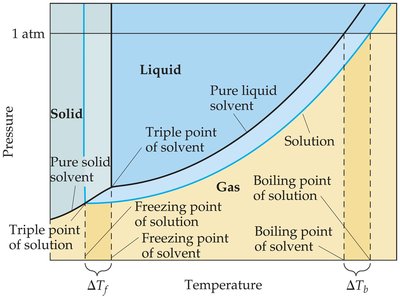
Adding a solute to a solvent stabilizes the liquid phase, resulting in a lower freezing point and a higher boiling point for the solution compared to the pure solvent.

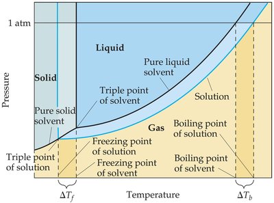
The magnitude of these effects depends on the concentration of solute particles, not their identity. For ionic compounds, the van’t Hoff factor (i) accounts for the number of particles produced upon dissociation.

• Boiling point elevation:

• Freezing point depression:

• Where and are the boiling and freezing point constants, respectively, and is the molality.

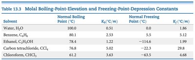
Boiling-Point Elevation and Freezing-Point Depression Constants

The values of and are specific to each solvent. The table below summarizes these constants for common solvents:

Application: Comparing Freezing Point Depression

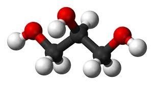
For three 0.15 m aqueous solutions: glycerin (C3H8O3), NaCl, and Zn(NO3)2:

• Glycerin is a nonelectrolyte ().

• NaCl dissociates into 2 ions ().

• Zn(NO3)2 dissociates into 3 ions ().

• The solution with the highest (Zn(NO3)2) will have the lowest freezing point.

Deviations in the van’t Hoff Factor

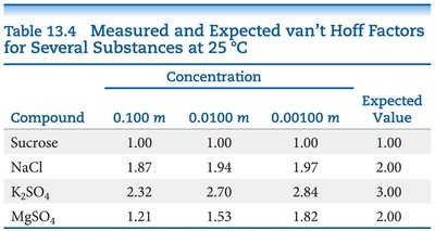
The van’t Hoff factor (i) is the ratio of the actual number of particles in solution after dissociation to the number of formula units dissolved. Deviations from expected values occur due to ion pairing and incomplete dissociation, especially at higher concentrations.

Example: The freezing point of a 0.05 m MgCl2 solution is measured to be −0.25°C. The van’t Hoff factor can be calculated and compared to expected values to assess the degree of dissociation.