Aggregate Expenditure and Output in the Short Run

Macroeconomic Equilibrium

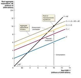
The aggregate expenditure (AE) model is a foundational concept in macroeconomics, used to determine the equilibrium level of real GDP in the short run. Macroeconomic equilibrium occurs where planned aggregate expenditure equals actual output (real GDP).

• Macroeconomic equilibrium is found at the intersection of the AE line and the 45° line, where AE = Y (real GDP).

• Any change in autonomous expenditure (expenditure not dependent on current income) shifts the AE line, altering equilibrium real GDP.

• Variables such as consumption (C), investment (I), government purchases (G), and net exports (NX) can change autonomous expenditure.

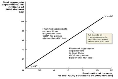
Additional info: The 45° line represents all points where AE equals real GDP. Only points on this line can be macroeconomic equilibrium.

Components of Aggregate Expenditure

The AE line is constructed by stacking the components of expenditure:

• Consumption (C): Spending by households on goods and services.

• Planned Investment (I): Spending by firms on capital goods.

• Government Purchases (G): Spending by the government on goods and services.

• Net Exports (NX): Exports minus imports.

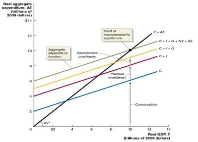
For simplicity, the model often assumes that I, G, and NX are autonomous (not affected by current real GDP).

The 45° Line Diagram

The 45° line diagram is a graphical tool to identify macroeconomic equilibrium:

• The 45° line shows all points where AE = Y.

• Points above the 45° line: AE > Y (planned spending exceeds output; inventories fall).

• Points below the 45° line: AE < Y (planned spending is less than output; inventories rise).

Shifts in Aggregate Expenditure and Policy Effects

Changes in autonomous expenditure shift the AE line, affecting equilibrium real GDP:

• Expansionary monetary policy (e.g., lower interest rates) increases investment and shifts AE upward, raising real GDP.

• Contractionary fiscal policy (e.g., lower government purchases or higher taxes) shifts AE downward, reducing real GDP.

• Increases in expected future income raise consumption, shifting AE upward and increasing real GDP.

Additional info: The AE model can be used to graphically show these shifts and their effects on equilibrium output.

The Multiplier Effect

The multiplier effect describes how an initial change in autonomous expenditure leads to a larger change in equilibrium real GDP.

• The multiplier is calculated as:

• Where MPC is the marginal propensity to consume (the fraction of additional income spent on consumption).

• The change in equilibrium real GDP is:

• The larger the MPC, the larger the multiplier.

• The multiplier effect works for both increases and decreases in autonomous expenditure.

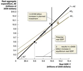
Example: If U.S. net exports rise by $100 billion and MPC = 0.8, the change in equilibrium real GDP is:

Limitations of the Multiplier

• The simple multiplier formula may overstate the actual effect because it ignores real-world factors such as changes in imports, inflation, interest rates, and taxes as GDP changes.

• In reality, the multiplier is often smaller than the theoretical value calculated from the MPC.

Business Cycles and Inventory Changes

Business cycles are influenced by changes in aggregate expenditure and inventories:

• A decline in one sector (e.g., residential construction) can reduce income and spending in other sectors due to the multiplier effect.

• Inventory drawdown refers to firms selling more than they produce, reducing inventories and signaling falling demand, which can lead to lower production and GDP.

• The impact of inventory changes on the business cycle depends on whether they are planned (intentional) or unplanned (unexpected).

Example: If firms experience unplanned inventory increases, it indicates that sales are lower than expected, leading firms to cut production and possibly triggering a recession.

Summary of Key Points

• Macroeconomic equilibrium occurs where AE = Y (on the 45° line).

• Shifts in autonomous expenditure change equilibrium real GDP.

• The multiplier effect amplifies changes in spending throughout the economy.

• The actual multiplier is often less than the theoretical value due to real-world complexities.

• Business cycles are affected by changes in spending, inventories, and expectations.