Chapter 4: Economic Efficiency, Government Price Setting, and Taxes

4.1 Consumer Surplus and Producer Surplus

This section introduces the concepts of consumer surplus and producer surplus, which measure the benefits that consumers and producers receive from participating in market transactions.

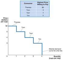
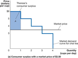
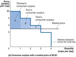
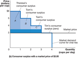
• Consumer Surplus: The difference between the highest price a consumer is willing to pay for a good or service and the actual price paid. It represents the net benefit to consumers.

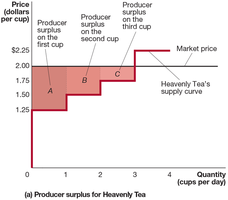
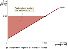
• Producer Surplus: The difference between the lowest price a firm would accept for a good or service (usually the marginal cost) and the price it actually receives. It represents the net benefit to producers.

• Marginal Benefit: The additional benefit to a consumer from consuming one more unit of a good or service.

• Marginal Cost: The change in a firm’s total cost from producing one more unit of a good or service.

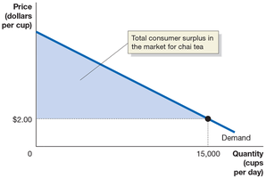
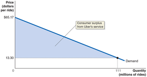
• Graphical Representation: Consumer surplus is the area below the demand curve and above the market price; producer surplus is the area above the supply curve and below the market price.

• Example: In the market for chai tea, if the price is $3.50, consumers whose willingness to pay is above $3.50 gain surplus. If the price falls, consumer surplus increases.

Formulas:

• Consumer Surplus (CS): $ CS = \sum_{i=1}^{n} (WTP_i - P) $

• Producer Surplus (PS): $ PS = \sum_{i=1}^{n} (P - MC_i) $

• For linear demand and supply: Area of triangle for CS or PS: $ \text{Area} = \frac{1}{2} \times \text{base} \times \text{height} $

4.2 The Efficiency of Competitive Markets

Economic efficiency in markets is achieved when resources are allocated in a way that maximizes total surplus (the sum of consumer and producer surplus). This occurs at the competitive equilibrium, where marginal benefit equals marginal cost.

• Economic Efficiency: A market outcome in which the marginal benefit to consumers of the last unit produced is equal to its marginal cost of production, and the sum of consumer and producer surplus is maximized.

• Deadweight Loss: The reduction in economic surplus resulting from a market not being in competitive equilibrium. It represents the lost gains from trade.

• Competitive Equilibrium: The point where the demand and supply curves intersect, indicating the most efficient allocation of resources.

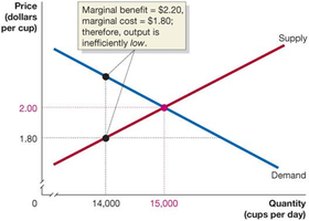
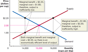
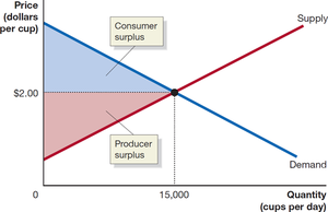
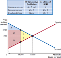
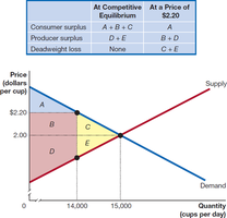
Formula:

• Economic Surplus (ES): $ ES = CS + PS $

• Deadweight Loss (DWL): $ DWL = \text{Potential ES at equilibrium} - \text{Actual ES} $

4.3 Government Intervention in the Market: Price Floors and Price Ceilings

Governments may intervene in markets by imposing price floors (minimum prices) or price ceilings (maximum prices). These interventions can lead to surpluses, shortages, and deadweight loss.

• Price Ceiling: A legally determined maximum price that sellers may charge (e.g., rent control).

• Price Floor: A legally determined minimum price that sellers may receive (e.g., minimum wage, agricultural price supports).

• Effects: Price floors can create surpluses (excess supply), while price ceilings can create shortages (excess demand).

• Deadweight Loss: Both price floors and ceilings reduce economic efficiency by creating deadweight loss.

• Winners and Losers: Some consumers or producers may benefit, while others lose. Illegal markets may arise when price controls are binding.

Example: Imposing a price floor in the wheat market raises the price but reduces the quantity traded, creating a surplus and deadweight loss.

Example: Rent ceilings lower rents for some but create shortages and reduce producer surplus.

Example: Minimum wage laws may increase incomes for some workers but reduce employment and create deadweight loss.

4.4 The Economic Effect of Taxes

Taxes are used by governments to raise revenue but can also affect market outcomes by shifting supply or demand curves, changing equilibrium prices and quantities, and creating deadweight loss.

• Per-Unit Tax: A tax assessed as a fixed dollar amount per unit sold (e.g., excise tax on gasoline).

• Tax Incidence: The actual division of the burden of a tax between buyers and sellers, determined by the relative elasticities of demand and supply, not by legal assignment.

• Deadweight Loss from Tax: Part of the consumer and producer surplus is lost due to the tax, and part is transferred to the government as tax revenue.

• Efficient Tax: A tax that raises revenue with minimal deadweight loss (excess burden).

Formulas:

• Tax Revenue: $ \text{Tax Revenue} = \text{Tax per unit} \times \text{Quantity sold after tax} $

• Deadweight Loss: $ DWL = \frac{1}{2} \times \text{Tax per unit} \times \text{Reduction in quantity sold} $

Appendix: Quantitative Demand and Supply Analysis

This section covers how to use equations for demand and supply to calculate equilibrium price and quantity, as well as the effects of government interventions such as rent controls.

• Equilibrium Condition: Set quantity demanded equal to quantity supplied and solve for price.

• Consumer and Producer Surplus: Use the area of triangles under the demand and above the supply curve to calculate surpluses.

• Deadweight Loss: Calculate the area representing lost surplus due to interventions like rent ceilings.

Formula for Area of a Triangle: $ \text{Area} = \frac{1}{2} \times \text{base} \times \text{height} $

Additional info: The above table summarizes the effects of a rent ceiling on consumer surplus, producer surplus, and deadweight loss, based on the quantitative analysis in the appendix.