Models, Positive and Normative Analysis, and Graphing

Introduction to Economic Models

Economic models are simplified representations of reality, designed to clarify the relationships between variables and to predict outcomes under specific assumptions. The process of modeling involves abstraction, classification of variables, and disciplined reasoning to ensure clarity and relevance.

• Purposeful Abstraction: Models omit unnecessary details to focus on essential mechanisms, following the principle of Ockham’s razor: use the simplest explanation adequate for the purpose.

• Variables: Models specify which factors are allowed to change (endogenous) and which are held constant or taken as given (exogenous).

• Ceteris Paribus: This Latin phrase means "other things equal" and is used to isolate the effect of one variable by holding others constant.

Endogenous and Exogenous Variables

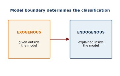
Every economic model distinguishes between endogenous and exogenous variables. This classification is determined by the model’s boundaries and purpose.

• Endogenous Variables: Explained within the model; their values are determined by the model’s structure.

• Exogenous Variables: Given outside the model; their values are imposed from the external environment.

• Model Boundary: The same variable can be endogenous in one model and exogenous in another, depending on the analytical focus.

Abstraction and Ockham’s Razor

Abstraction is the deliberate omission of detail to highlight the essential relationship. Ockham’s razor guides economists to prefer simpler models unless additional complexity improves explanation or prediction.

• Disciplined Abstraction: Begins with a minimal set of variables and adds detail only if it changes the model’s implications.

• Purpose-Driven Detail: The appropriate level of detail depends on the question being addressed.

Ceteris Paribus: Controlled Comparison

Ceteris paribus is a foundational concept in economic reasoning, allowing for the isolation of the effect of one variable by holding others constant. This approach clarifies the conditional nature of economic predictions.

• Conditional Predictions: The effect described is valid only if the held-constant factors do not change.

• Limits of Application: Real-world changes in the held-constant variables require re-examination of the model’s predictions.

Claims and Policy Criteria

Positive vs. Normative Analysis

Economic analysis distinguishes between positive (descriptive or predictive) and normative (prescriptive or evaluative) claims.

• Positive Analysis: Describes how the economy works or predicts outcomes; can be tested against evidence.

• Normative Analysis: Involves value judgments about what ought to be; depends on criteria such as fairness, efficiency, or equity.

• Policy Arguments: Often combine both types; separating them clarifies the basis for disagreement.

Policy Criteria

Policy recommendations require explicit criteria for judging outcomes. Common criteria include:

• Efficiency: Achieving the maximum output with given resources.

• Equity: Fair distribution of income, wealth, or opportunities.

• Growth: Expansion of productive capacity and output.

• Stability: Avoiding large fluctuations in output, employment, or prices.

Transparent analysis reports effects under multiple criteria and explains whose outcomes are considered, over what time horizon, and under what uncertainties.

Empirical Testing and Causal Reasoning

Empirical Testing

Empirical economics uses data to evaluate models and theories. The process involves defining measurable variables, making predictions, and designing comparisons that can support or refute the model.

• Measurement: Careful definition of variables, units, and populations is essential.

• Comparison: Observations are compared across groups, places, or time periods to test predictions.

• Revision: Models are revised in light of evidence, improving accuracy and relevance.

Correlation vs. Causation

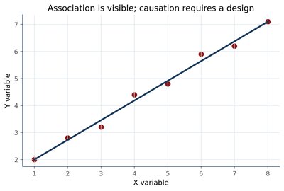
Correlation means two variables move together, but does not imply one causes the other. Establishing causation requires careful research design to rule out alternative explanations and confounding factors.

• Confounding: A third variable may influence both variables of interest, creating a spurious association.

• Counterfactual: Causal claims require comparison to what would have happened in the absence of the suspected cause.

• Research Design: Methods such as random assignment, natural experiments, and statistical controls help approximate the counterfactual.

Research Design and Validity

Good research design strengthens causal inference by approximating the missing counterfactual and clarifying the limits of the evidence.

• Internal Validity: Whether the study identifies an effect in the examined setting.

• External Validity: Whether the result generalizes to other settings.

• Transparency: Credible studies explain their limitations and the assumptions underlying their conclusions.

Graphs as Economic Language

Time-Series Graphs

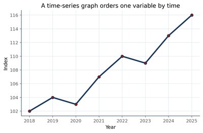
A time-series graph displays the value of a variable over time, with time on the horizontal axis and the variable of interest on the vertical axis. These graphs reveal trends, cycles, and unusual observations but do not explain causes by themselves.

• Interpretation: Requires attention to frequency, units, and the meaning of each observation.

• Limitations: Interpolation and extrapolation beyond observed data are uncertain.

Two-Variable Graphs: Axes, Intercepts, and Relationships

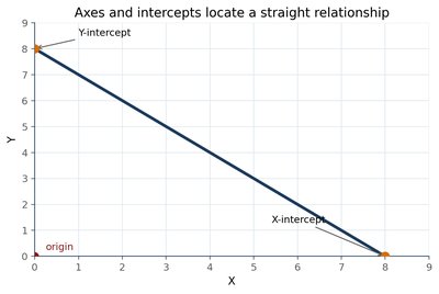
Two-variable graphs are fundamental tools in economics, with the independent variable on the X-axis and the dependent variable on the Y-axis. Key features include the origin, intercepts, and the direction of the relationship.

• Y-Intercept: Where the line crosses the Y-axis (X = 0).

• X-Intercept: Where the line crosses the X-axis (Y = 0).

• Positive Relationship: Upward-sloping line; as X increases, Y increases.

• Negative Relationship: Downward-sloping line; as X increases, Y decreases.

Slope: Definition and Cases

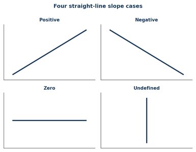
The slope of a line measures the change in the Y variable per unit change in the X variable ("rise over run"). Four cases exhaust the possibilities for straight lines:

• Positive Slope: Variables move together (upward-sloping).

• Negative Slope: Variables move in opposite directions (downward-sloping).

• Zero Slope: Horizontal line; Y does not respond to X.

• Undefined/Infinite Slope: Vertical line; X does not change, Y changes.

For curved lines, the slope changes at each point, which is important for modeling diminishing returns and other nonlinear relationships.

Movement Along vs. Shift of a Curve

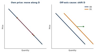
Distinguishing between movement along a curve and a shift of the entire curve is a critical skill in economic graph interpretation.

• Movement Along the Curve: Caused by a change in a variable on one of the axes (e.g., price for a demand curve).

• Shift of the Curve: Caused by a change in a variable not on the axes (e.g., income, tastes, or the price of related goods for a demand curve).

• Rule: If the changing variable is on an axis, move along the curve; if not, shift the curve.

Graph-Reading Precautions

Accurate graph interpretation requires careful attention to variables, units, scales, and the relevant domain. Visual impressions can be misleading if the scale is manipulated or if omitted variables and confounding factors are not considered.

• Axis Construction: Check if scales start at zero, intervals are equal, and whether transformations are used.

• Domain: Interpret only within the range supported by data and assumptions.

• Magnitude vs. Visual Steepness: Economic importance depends on actual values, not just how steep a line appears.

Summary Table: Key Concepts in Economic Modeling

Additional info: These notes expand on the lecture content with definitions, examples, and structured explanations to provide a comprehensive foundation for understanding economic modeling, analysis, and graphing in microeconomics.