Elasticity and Its Application

Introduction to Elasticity

Elasticity is a fundamental concept in microeconomics that measures how responsive the quantity demanded or supplied of a good is to changes in its determinants, such as price, income, or the price of related goods. Understanding elasticity helps businesses and policymakers predict the effects of price changes, taxation, and market shifts.

Price Elasticity of Demand

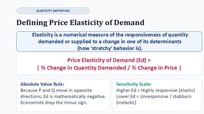
Defining Price Elasticity of Demand

Price Elasticity of Demand (Ed) quantifies the responsiveness of quantity demanded to a change in price. It is calculated as:

• Absolute Value Rule: Price and quantity move in opposite directions, so Ed is mathematically negative. Economists use the absolute value.

• Sensitivity Scale: Higher Ed means demand is highly responsive (elastic); lower Ed means demand is unresponsive (inelastic).

Business Scenario: Pricing Dilemma

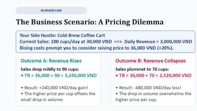
Elasticity is crucial for pricing decisions. For example, a coffee cart owner considers raising prices due to rising costs. The outcome depends on how customers respond:

• Outcome A: Revenue rises if the drop in sales is small compared to the price increase.

• Outcome B: Revenue collapses if the drop in sales is large, overwhelming the price increase.

The Midpoint Method

Why We Need the Midpoint Method

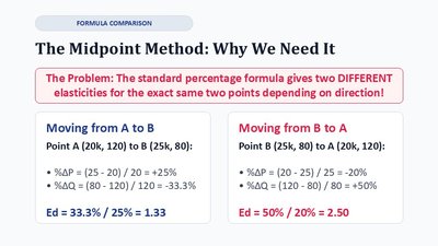
The standard percentage formula for elasticity can yield different results depending on the direction of calculation. The midpoint method solves this by using averages, ensuring consistency.

• Moving from A to B:

• Moving from B to A:

The Midpoint Formula (Universal Standard)

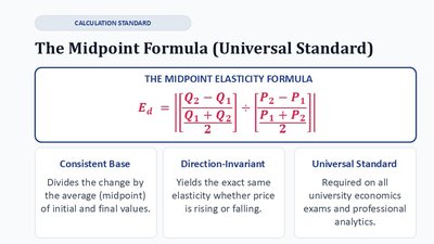
The midpoint formula is the universal standard for calculating elasticity:

• Consistent Base: Uses the average of initial and final values.

• Direction-Invariant: Yields the same elasticity whether price is rising or falling.

• Universal Standard: Required in university exams and analytics.

Calculating Elasticity: Active Learning Example

Step-by-Step Calculation

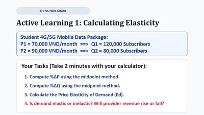
Given a change in price and quantity for a mobile data package:

• Price rises from 70,000 VND to 90,000 VND; subscribers fall from 120,000 to 80,000.

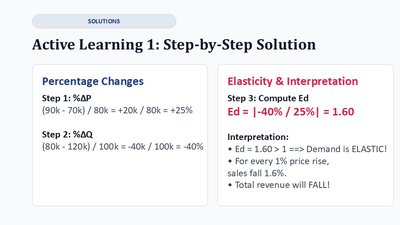
• Calculate percentage changes using the midpoint method:

• Compute Ed:

• Interpretation: Demand is elastic; total revenue will fall.

Determinants of Price Elasticity of Demand

Four Key Drivers

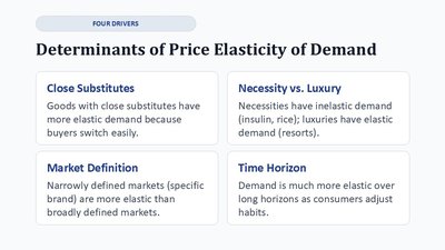
• Close Substitutes: More substitutes increase elasticity.

• Necessity vs. Luxury: Necessities are inelastic; luxuries are elastic.

• Market Definition: Narrowly defined markets are more elastic.

• Time Horizon: Demand is more elastic in the long run.

The Spectrum of Demand Curves

Categories of Elasticity

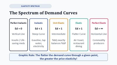
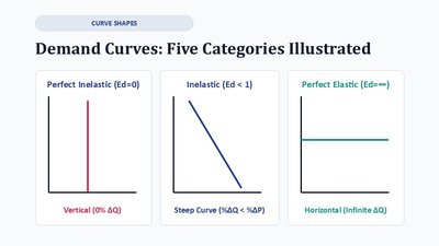
• Perfect Inelastic (Ed = 0): Vertical line; quantity does not change.

• Inelastic (Ed < 1): Steep curve; quantity changes less than price.

• Unit Elastic (Ed = 1): Intermediate; %ΔQ exactly balances %ΔP.

• Elastic (Ed > 1): Flatter curve; quantity changes more than price.

• Perfect Elastic (Ed = ∞): Horizontal line; quantity changes infinitely with price.

Elasticity Along a Linear Demand Curve

Elasticity vs. Slope

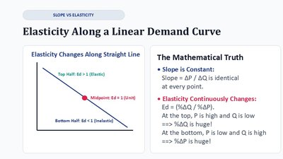
While the slope of a linear demand curve is constant, elasticity changes along the curve:

• At the top, price is high and quantity is low: Ed is large (elastic).

• At the bottom, price is low and quantity is high: Ed is small (inelastic).

• Midpoint: Ed = 1 (unit elastic).

Elasticity and Total Revenue

Relationship Between Elasticity and Total Revenue

Total Revenue (TR) is calculated as price times quantity (). The effect of price changes on TR depends on elasticity:

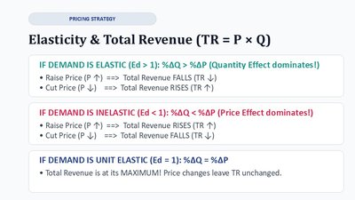
• If demand is elastic (Ed > 1): Raising price decreases TR; cutting price increases TR.

• If demand is inelastic (Ed < 1): Raising price increases TR; cutting price decreases TR.

• If demand is unit elastic (Ed = 1): TR is maximized; price changes do not affect TR.

Active Learning: Pricing Strategy Challenge

Examples

• University Tuition: Inelastic demand (Ed = 0.45); raising tuition increases total revenue.

• Vacation Airfares: Elastic demand (Ed = 1.80); cutting fares increases total revenue.

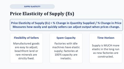
Price Elasticity of Supply

Definition and Determinants

Price Elasticity of Supply (Es) measures how easily and quickly sellers can adjust output when prices change:

• Flexibility of Sellers: Manufactured goods are more elastic; fixed resources are inelastic.

• Spare Capacity: Idle machines increase elasticity; full capacity is inelastic.

• Time Horizon: Supply is more elastic in the long run.

Income and Cross-Price Elasticities

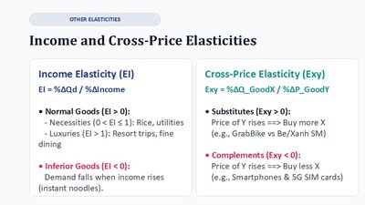
Income Elasticity (EI)

Measures how demand changes as consumer income changes:

• Normal Goods (EI > 0): Demand rises with income.

• Inferior Goods (EI < 0): Demand falls as income rises.

Cross-Price Elasticity (Exy)

Measures how demand for one good responds to price changes in another:

• Substitutes (Exy > 0): Price of Y rises, demand for X rises.

• Complements (Exy < 0): Price of Y rises, demand for X falls.

Applications of Elasticity

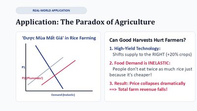
The Paradox of Agriculture

High-yield technology increases supply, but if food demand is inelastic, prices collapse and total farm revenue falls.

Public Health & Sin Taxes

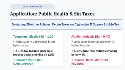
Elasticity informs policy design for excise taxes. For example, teenagers' demand for cigarettes is elastic, so taxes cut consumption. Adults' demand is inelastic, so taxes raise revenue.

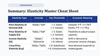
Summary: Elasticity Master Cheat Sheet