Firms and Production

Production Functions and Inputs

In microeconomics, firms transform inputs into outputs using technology. The production function describes this relationship mathematically.

• Production Function: , where q is output, L is labor, and K is capital.

• Isoquant Curve: A set of input bundles that produce the same output.

• Isoquant Map: Collection of isoquant curves for different output levels.

• Short Run: Some inputs (e.g., labor) are adjustable, others (e.g., capital) are fixed.

• Long Run: All inputs are adjustable.

Example: A factory may adjust labor daily but can only change machinery over years.

Costs

Short-Run Cost Functions

Short-run costs are divided into fixed and variable components. The cost functions help firms decide how much to produce.

• Fixed Cost (FC): Costs that do not change with output (e.g., rent).

• Variable Cost (VC): Costs that change with output (e.g., wages).

• Total Cost (TC):

• Marginal Cost (MC):

• Average Cost (AC):

• Average Variable Cost (AVC):

• Average Fixed Cost (AFC):

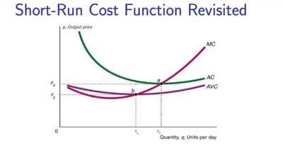
Typical Properties: AC and AVC are U-shaped. MC intersects AC and AVC at their minimum points.

Long-Run Cost Functions

In the long run, all inputs are variable. The long-run average cost (LRAC) and long-run marginal cost (LRMC) are key concepts.

• Long-Run Cost Function:

• Long-Run Average Cost:

• Long-Run Marginal Cost:

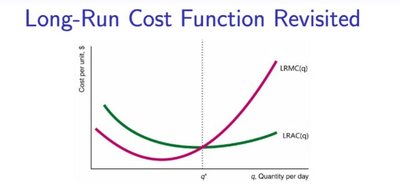
• LRAC is U-shaped: Decreases due to economies of scale, then increases due to diseconomies.

• Relationship:

  • When :

  • When :

  • When :

Supply Curves

Short-Run Individual Supply Curve

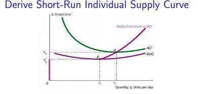
The short-run supply curve is the portion of the MC curve above AVC. Producers supply output where price is greater than or equal to AVC.

• Shut-down Price (): If , supply is zero.

• Break-even Price (): If , producer earns zero profit.

• Supply Decision: If , produce where .

Long-Run Individual Supply Curve

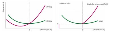
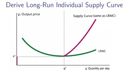
The long-run supply curve is the portion of the LRMC curve above LRAC. In the long run, producers can enter or exit freely.

• Long-Run Shut-down Price (): If , supply is zero.

• Break-even Price: is both shut-down and break-even price in the long run.

• Supply Decision: If , produce where .

Market Supply Curve

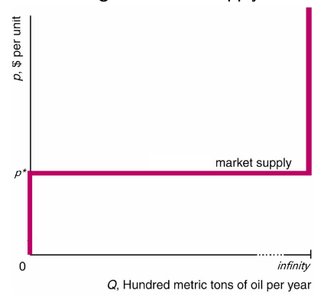
The market supply curve aggregates individual supply curves. In the long run, the supply curve is horizontal at the break-even price if there are infinitely many identical producers.

• Short Run: Sum individual supply curves for given producers.

• Long Run: Entry and exit lead to a horizontal supply curve at .

Economic Surplus

Producer Surplus (PS)

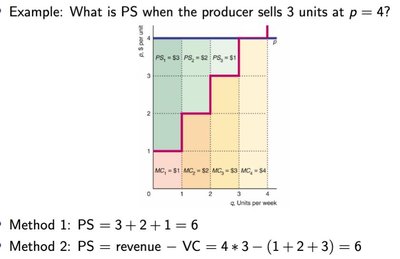
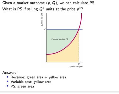
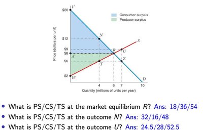
Producer surplus is the gain from trade for producers, calculated as revenue minus variable cost.

• PS Calculation: Two methods:

  • Sum marginal gains unit by unit.

  • PS = Revenue - VC

Consumer Surplus (CS)

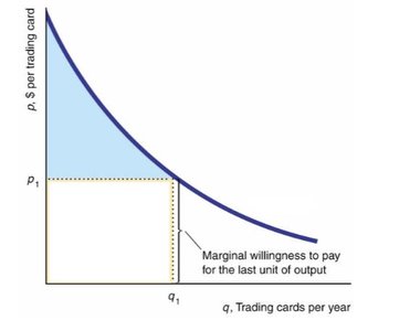
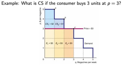
Consumer surplus is the gain from trade for consumers, calculated as willingness to pay minus expenditure.

• Marginal Willingness to Pay (MWTP): The demand curve represents MWTP.

• CS Calculation: Two methods:

  • Sum marginal gains unit by unit.

  • CS = WTP - Expenditure

Total Surplus (TS)

Total surplus is the sum of producer and consumer surplus, representing social welfare.

• TS Formula:

• Market Equilibrium: Maximizes total surplus when MWTP = MC.

Market Interventions

Tax

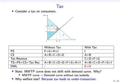
A tax reduces the quantity traded, leading to deadweight loss and lower total surplus.

• Tax Revenue: Collected by government.

• Deadweight Loss (DWL): Lost surplus due to under-transaction.

Subsidy

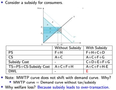
A subsidy increases the quantity traded, leading to deadweight loss from over-transaction.

• Subsidy Cost: Paid by government.

• Deadweight Loss (DWL): Lost surplus due to over-transaction.

Price Controls

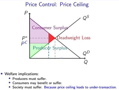
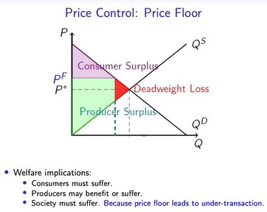
Price ceilings and floors cause deadweight loss by restricting market transactions.

• Price Ceiling: Maximum price allowed; leads to under-transaction.

• Price Floor: Minimum price allowed; also leads to under-transaction.

Import Ban and Tariff

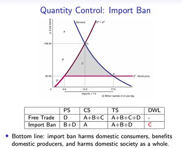
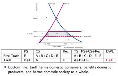
Import bans and tariffs restrict trade, harming consumers and society overall, but benefiting domestic producers.

Externalities

Negative Externalities

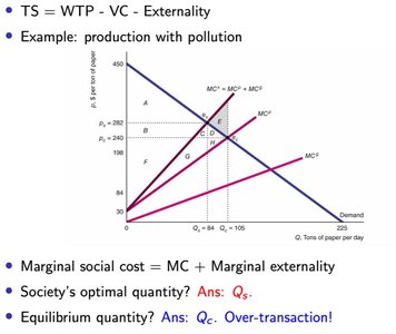
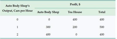
Negative externalities occur when a producer or consumer's actions harm others. The market equilibrium typically results in over-transaction compared to the social optimum.

• Marginal Social Cost: Marginal externality

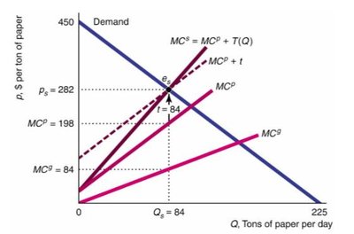
• Remedies: Property rights (market approach), taxes, or quantity controls (regulation approach).

Positive Externalities

Positive externalities occur when actions benefit others. The market equilibrium results in under-transaction compared to the social optimum.

• Marginal Social Benefit: Marginal externality

• Remedies: Property rights (market approach), subsidies, government provision, or mandates (regulation approach).

Summary Table: Key Formulas

• Average Product of Labor:

• Profit:

• Short-Run Total Cost:

• Long-Run Average Cost:

• Producer Surplus:

• Consumer Surplus:

• Total Surplus:

Additional info: All diagrams and tables included are directly relevant to the explanation of the adjacent paragraphs, visually reinforcing key microeconomic concepts.