Solving Demand and Supply Equations

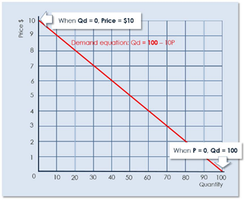
Linear Demand and Supply Functions

In microeconomics, demand and supply are often represented as linear equations. These equations allow us to analyze how price and quantity interact in a market, and to solve for equilibrium where demand equals supply.

• Demand Equation (in terms of Price):

• Demand Equation (in terms of Quantity):

• Supply Equation (in terms of Price):

• Supply Equation (in terms of Quantity):

Key Terms:

• Vertical Intercept: The value where the line crosses the price axis (a for demand, c for supply).

• Slope: The rate at which price changes with quantity (b for demand, d for supply).

• Horizontal Intercept: The value where the line crosses the quantity axis ( for demand, for supply).

• Inverse Slope: for demand, for supply.

Market Equilibrium

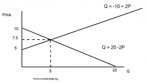
Market equilibrium occurs where the quantity demanded equals the quantity supplied at a particular price. This is the point at which the market clears, and there is no surplus or shortage.

• Equilibrium Condition:

• Solving for Equilibrium: Set the demand and supply equations equal to each other and solve for price and quantity.

Example:

• Given: and

• Set :

• Combine terms:

• Substitute back:

Tabular Approach to Market Equilibrium

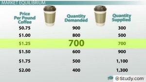
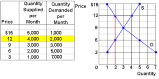
Market equilibrium can also be found using tables that list prices, quantities demanded, and quantities supplied. The equilibrium is where the quantity demanded equals the quantity supplied.

Example: At a price where quantity demanded equals quantity supplied, the market is in equilibrium.

Graphical Representation of Demand and Supply

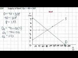
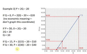
Demand and supply curves can be plotted on a graph, with price on the vertical axis and quantity on the horizontal axis. The intersection of the curves represents the equilibrium price and quantity.

• Demand Curve: Downward sloping, showing inverse relationship between price and quantity demanded.

• Supply Curve: Upward sloping, showing direct relationship between price and quantity supplied.

• Equilibrium Point: Intersection of demand and supply curves.

Practice Problems

Solving for equilibrium price and quantity is a fundamental skill in microeconomics. Practice problems often involve setting up and solving linear equations for demand and supply.

• Using the Demand Equation: and the Supply Equation: , solve for equilibrium price and quantity.

• Using the Inverse Demand Equation: and the Inverse Supply Equation: , solve for equilibrium price and quantity. Also plot the graph, labeling axes and equilibrium.

• Using the Inverse Demand Equation: and the Inverse Supply Equation: , solve for equilibrium price and quantity. Also plot the graph, labeling axes and equilibrium.

Example Solution:

• Set and solve for .

• Substitute back into either equation to find .

Additional info: Graphs and tables are essential for visualizing market equilibrium and understanding the relationship between price and quantity in microeconomic models.