Indietro
Study Guide: The Market Forces of Supply and Demand in Microeconomics
Guida di studio - Note intelligenti
 Appunti personalizzati basati sui tuoi materiali, ampliati con definizioni chiave, esempi e contesto.
The Market Forces of Supply and Demand
Introduction
This section explores the fundamental principles of microeconomics, focusing on how buyers and sellers interact in markets to determine prices and quantities. Key concepts include the law of demand and supply, market equilibrium, and comparative statics.
What Is a Market?
Definition and Types
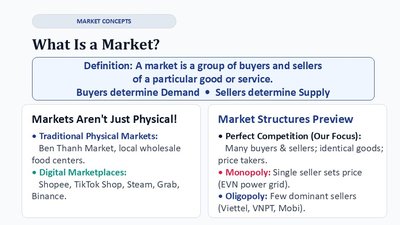
A market is a group of buyers and sellers of a particular good or service. Buyers determine demand, while sellers determine supply. Markets can be physical (e.g., local wholesale food centers) or digital (e.g., Shopee, Steam, Binance).
Traditional Physical Markets: Ben Thanh Market, local food centers.
Digital Marketplaces: Shopee, TikTok Shop, Steam, Grab, Binance.
Market Structures Preview
Perfect Competition: Many buyers and sellers, identical goods, price takers.
Monopoly: Single seller sets price (e.g., EVN power grid).
Oligopoly: Few dominant sellers (e.g., Viettel, VNPT, Mobi).
Demand: The Buyer's Perspective
The Law of Demand
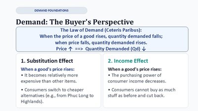
The Law of Demand (ceteris paribus): When the price of a good rises, quantity demanded falls; when price falls, quantity demanded rises.
Substitution Effect: Higher prices make alternatives more attractive.
Income Effect: Higher prices reduce purchasing power.
The Demand Schedule and Demand Curve
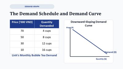
A demand schedule lists quantities demanded at various prices. The demand curve is downward-sloping, reflecting the inverse relationship between price and quantity demanded.
Price ('000 VND) | Quantity Demanded |
|---|---|
70 | 4 cups |
50 | 8 cups |
30 | 12 cups |
10 | 16 cups |
Market Demand: Horizontal Summation
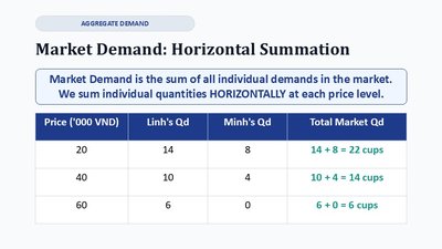
Market demand is the sum of all individual demands at each price level. Quantities are summed horizontally.
Price ('000 VND) | Linh's Qd | Minh's Qd | Total Market Qd |
|---|---|---|---|
20 | 14 | 8 | 22 cups |
40 | 10 | 4 | 14 cups |
60 | 6 | 0 | 6 cups |
Shifts in Demand vs. Movements Along
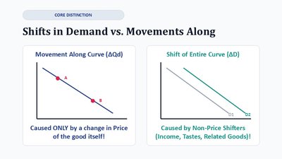
Movement along the curve is caused by price changes. Shifts of the curve are caused by non-price factors (income, tastes, related goods).
Non-Price Determinants of Demand (Shifters)
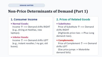
Consumer Income: Normal goods (demand shifts right with income rise); Inferior goods (demand shifts left with income rise).
Prices of Related Goods: Substitutes (demand shifts right if substitute price rises); Complements (demand shifts left if complement price rises).
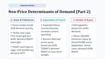
Tastes & Preferences: Trends and health warnings can shift demand.
Expectations of Future: Anticipated changes in income or prices affect current demand.
Number of Buyers: Demographic changes shift demand.
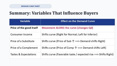
Summary Table: Variables That Influence Buyers
Variable | Effect on the Demand Curve |
|---|---|
Price of the good itself | Movement ALONG the curve (changes Qd) |
Consumer Income | Shifts curve (Right for Normal; Left for Inferior) |
Price of a Substitute | Shifts curve (Price of Sub ↑ ⇒ Demand shifts Right) |
Price of a Complement | Shifts curve (Price of Comp ↑ ⇒ Demand shifts Left) |
Tastes & Expectations | Shifts curve (Favorable taste / expected rise ⇒ Shifts Right) |
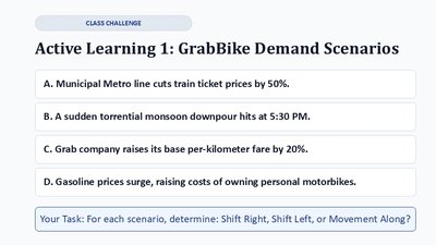
Active Learning: Demand Scenarios
Students analyze scenarios to determine if demand shifts right, left, or if there is movement along the curve.
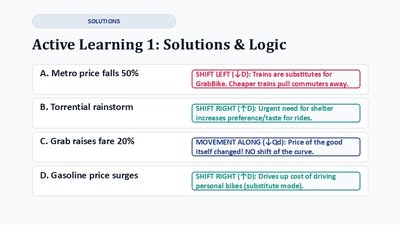
A. Metro price falls 50%: Shift Left (trains are substitutes).
B. Torrential rainstorm: Shift Right (urgent need increases preference).
C. Grab raises fare 20%: Movement Along (price change).
D. Gasoline price surges: Shift Right (drives up cost of substitutes).
Supply: The Seller's Perspective
The Law of Supply
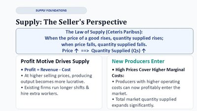
The Law of Supply (ceteris paribus): When the price of a good rises, quantity supplied rises; when price falls, quantity supplied falls.
Profit Motive: Higher prices increase profit margins, motivating increased production.
New Producers Enter: High prices cover higher marginal costs, attracting new suppliers.
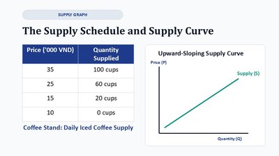
The Supply Schedule and Supply Curve
A supply schedule lists quantities supplied at various prices. The supply curve is upward-sloping, reflecting the direct relationship between price and quantity supplied.
Price ('000 VND) | Quantity Supplied |
|---|---|
35 | 100 cups |
25 | 60 cups |
15 | 20 cups |
10 | 0 cups |
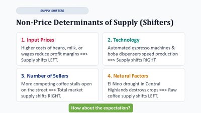
Non-Price Determinants of Supply (Shifters)
Input Prices: Higher costs shift supply left.
Technology: Improved technology shifts supply right.
Number of Sellers: More sellers shift supply right.
Natural Factors: Adverse events (e.g., drought) shift supply left.
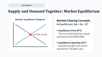
Market Equilibrium
Supply and Demand Together
Market equilibrium occurs where quantity demanded equals quantity supplied (Qd = Qs = Q*). The equilibrium price (P*) balances supply and demand.
Equilibrium Price (P*): The price at which Qd = Qs.
Equilibrium Quantity (Q*): The quantity bought and sold at equilibrium.
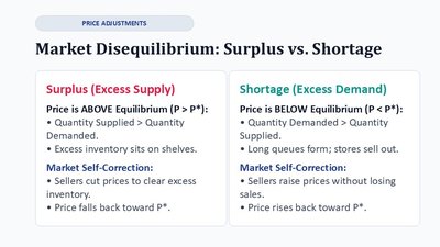
Market Disequilibrium: Surplus vs. Shortage
Surplus (Excess Supply): Price above equilibrium; quantity supplied exceeds quantity demanded.
Shortage (Excess Demand): Price below equilibrium; quantity demanded exceeds quantity supplied.
Market Self-Correction: Prices adjust to restore equilibrium.
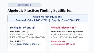
Algebraic Practice: Finding Equilibrium
Equilibrium can be found by setting Qd = Qs and solving for P* and Q* using market equations.
Given: Demand ; Supply
Set and solve for P*:
Find :
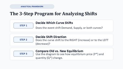
Analyzing Shifts: The 3-Step Program
Framework for Comparative Statics
Step 1: Decide which curve shifts (demand, supply, or both).
Step 2: Decide shift direction (right/increase or left/decrease).
Step 3: Compare old vs. new equilibrium (P*, Q* change).
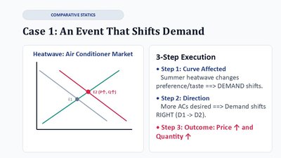
Comparative Statics: Single Shifts
Case 1: Event That Shifts Demand
Example: Summer heatwave increases demand for air conditioners. Demand curve shifts right, leading to higher equilibrium price and quantity.
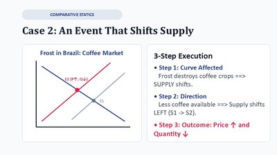
Case 2: Event That Shifts Supply
Example: Frost destroys coffee crops in Brazil. Supply curve shifts left, leading to higher equilibrium price and lower equilibrium quantity.
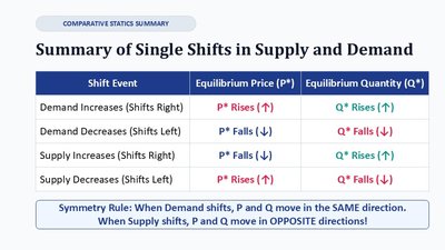
Summary Table: Single Shifts in Supply and Demand
Shift Event | Equilibrium Price (P*) | Equilibrium Quantity (Q*) |
|---|---|---|
Demand Increases (Right) | P* Rises (↑) | Q* Rises (↑) |
Demand Decreases (Left) | P* Falls (↓) | Q* Falls (↓) |
Supply Increases (Right) | P* Falls (↓) | Q* Rises (↑) |
Supply Decreases (Left) | P* Rises (↑) | Q* Falls (↓) |
Simultaneous Shifts: The Ambiguity Trap
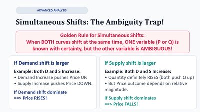
Golden Rule for Simultaneous Shifts
When both curves shift, one variable (P or Q) is known with certainty, but the other is ambiguous. The outcome depends on the relative magnitude of shifts.
If demand shift is larger: Price rises.
If supply shift is larger: Price falls.
The Simultaneous Shift Matrix
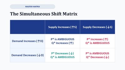
Supply Increases (↑S) | Supply Decreases (↓S) | |
|---|---|---|
Demand Increases (↑D) | P* is AMBIGUOUS, Q* Increases (↑) | P* Increases (↑), Q* is AMBIGUOUS |
Demand Decreases (↓D) | P* Decreases (↓), Q* is AMBIGUOUS | P* is AMBIGUOUS, Q* Decreases (↓) |
Real-World Application: Electric Motorbike Shock
Analyzing Shifts
Event 1: Heavy public subsidies shift demand to the right (↑D).
Event 2: Battery technology cuts shift supply to the right (↑S).
Market Equilibrium Result
Quantity (Q*): Both shifts increase quantity; Q* definitely rises.
Price (P*): Demand pulls price up, supply pushes price down; outcome is ambiguous.

Conclusion: How Prices Allocate Scarce Resources
The Price Mechanism in Action
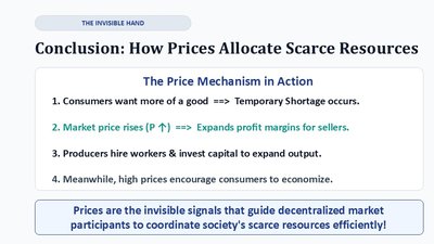
Temporary shortages occur when consumers want more of a good.
Market price rises, expanding profit margins for sellers.
Producers hire workers and invest capital to expand output.
High prices encourage consumers to economize.
Prices are the invisible signals that guide decentralized market participants to coordinate society's scarce resources efficiently.