Application — The Costs of Taxation

Introduction

This chapter explores the economic consequences of taxation, focusing on deadweight loss, tax distortion, and the Laffer Curve. It analyzes how taxes affect market equilibrium, social welfare, and government revenue, providing both theoretical and real-world perspectives.

The Anatomy of a Tax Wedge

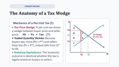
Mechanics of a Per-Unit Tax

• The Price Wedge: A per-unit tax creates a gap between the price buyers pay (Pb) and the price sellers receive (Ps). The wedge equals the tax amount (T):

• Traded Quantity Shrinks: The tax reduces the equilibrium quantity from Q* to Qt because buyers pay more and sellers receive less.

• Statutory Equivalence: The economic outcome is identical whether the tax is levied on buyers or sellers.

Welfare Effects of a Per-Unit Tax

Social Surplus and Deadweight Loss

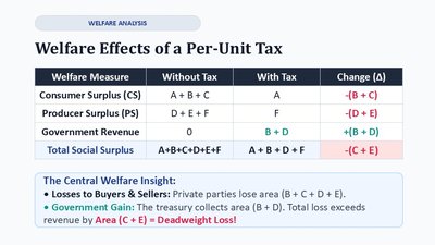
• Consumer Surplus (CS): Falls by area B + C.

• Producer Surplus (PS): Falls by area D + E.

• Government Revenue: Gains area B + D.

• Total Social Surplus: Falls by area C + E, which is the deadweight loss (DWL).

Visualizing Tax Revenue & Deadweight Loss

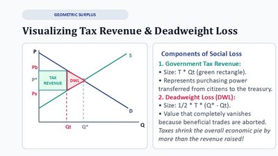
Components of Social Loss

• Government Tax Revenue: (green rectangle). Represents purchasing power transferred from citizens to the treasury.

• Deadweight Loss (DWL): (triangle). Represents lost mutual gains from trade due to prevented transactions.

What Causes Deadweight Loss?

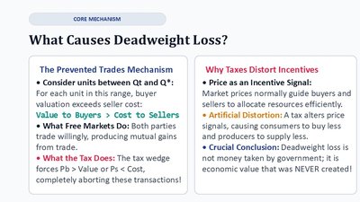
The Prevented Trades Mechanism

• For units between Qt and Q*, buyer value exceeds seller cost, but the tax wedge prevents these trades.

• Free Markets: All mutually beneficial trades occur.

• With Tax: Tax wedge aborts these transactions, causing deadweight loss.

Why Taxes Distort Incentives

• Price as an Incentive Signal: Taxes alter price signals, causing consumers and producers to change behavior.

• Artificial Distortion: Deadweight loss is not money taken by government; it is economic value that never existed.

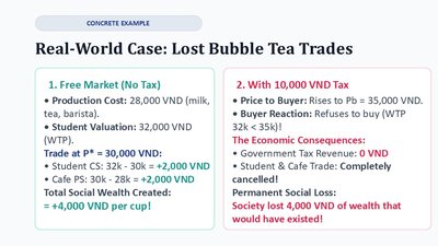
Real-World Example: Lost Bubble Tea Trades

Case Study

• Free Market (No Tax): Production cost = 28,000 VND; student valuation = 32,000 VND; trade at 30,000 VND creates 4,000 VND of social wealth per cup.

• With 10,000 VND Tax: Price rises to 35,000 VND; buyer refuses to buy; trade is cancelled; government revenue = 0; permanent social loss = 4,000 VND per cup.

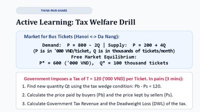
Active Learning: Tax Welfare Drill

Market for Bus Tickets

• Demand: P = 800 - 2Q

• Supply: P = 200 + 4Q

• Free Market Equilibrium: P* = 600 ('000 VND), Q* = 100 thousand tickets

• Tax Imposed: T = 120 ('000 VND) per ticket

1. Find new quantity Qt using tax wedge: Pb - Ps = 120

2. Calculate Pb (price paid by buyers) and Ps (price received by sellers)

3. Calculate government tax revenue and deadweight loss

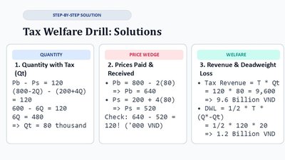
Step-by-Step Solution

• Quantity with Tax: thousand

• Prices Paid & Received: Check: ('000 VND)

• Revenue & Deadweight Loss: Tax Revenue: Billion VND DWL: Billion VND

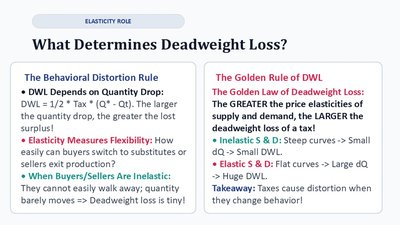
What Determines Deadweight Loss?

The Behavioral Distortion Rule

• DWL depends on the drop in quantity:

• Elasticity Measures Flexibility: The more easily buyers and sellers can substitute or exit, the larger the quantity drop and the greater the lost surplus.

• Inelastic Markets: Quantity barely changes; DWL is tiny.

The Golden Rule of DWL

• The greater the price elasticities of supply and demand, the larger the deadweight loss of a tax.

• Inelastic S & D: Steep curves → Small dQ → Small DWL

• Elastic S & D: Flat curves → Large dQ → Huge DWL

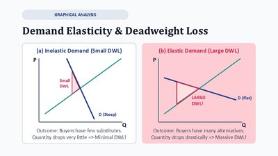
Demand Elasticity & Deadweight Loss

Graphical Analysis

• Inelastic Demand: Steep demand curve; buyers have few substitutes; quantity drops very little; minimal DWL.

• Elastic Demand: Flat demand curve; buyers have many alternatives; quantity drops drastically; massive DWL.

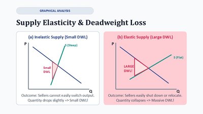
Supply Elasticity & Deadweight Loss

Graphical Analysis

• Inelastic Supply: Steep supply curve; sellers cannot easily switch output; quantity drops slightly; small DWL.

• Elastic Supply: Flat supply curve; sellers easily shut down or relocate; quantity collapses; massive DWL.

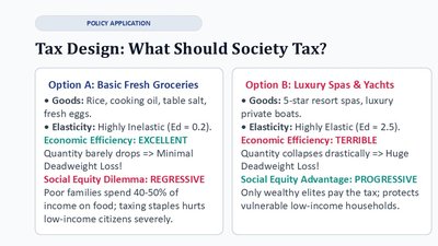
Tax Design: What Should Society Tax?

Policy Application

• Option A: Basic Fresh Groceries Goods: Rice, cooking oil, table salt, fresh eggs Elasticity: Highly inelastic (Ed = 0.2) Economic Efficiency: Excellent (minimal DWL) Social Equity Dilemma: Regressive (hurts low-income families)

• Option B: Luxury Spas & Yachts Goods: 5-star resort spas, luxury private boats Elasticity: Highly elastic (Ed = 2.5) Economic Efficiency: Terrible (huge DWL) Social Equity Advantage: Progressive (targets wealthy)

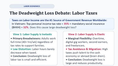
The Deadweight Loss Debate: Labor Taxes

Labor Economics

• Taxes on Labor Income: Major source of government revenue worldwide.

• View 1: Labor Supply Is Inelastic: Adults work full-time regardless of tax rates; low distortion; DWL is small.

• View 2: Labor Supply Is Elastic: Overtime, gig work, migration; taxes push talent abroad; DWL is large and reduces productivity.

How Tax Size Multiplies Deadweight Loss

Non-Linear Growth

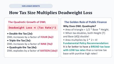
• Quadratic Growth of DWL: Doubling the tax increases DWL by a factor of four; tripling by nine; quadrupling by sixteen.

• Golden Rule of Public Finance: Broad tax base with low rates is preferable to narrow base with high rates.

The Laffer Curve: Tax Size vs. Revenue

Supply-Side Economics

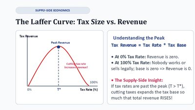
• Tax Revenue Formula:

• At 0% tax rate, revenue is zero; at 100% tax rate, revenue is zero (no legal activity).

• Supply-Side Insight: If tax rates exceed the peak, cutting rates can increase total revenue.

Case Study: Supply-Side Economics

Policy Case Study

• Reagan's 1980s Tax Cuts: Claimed to stimulate work and investment; total revenue did not rise, but rich earners paid more because they stopped using tax shelters.

• Vietnam Corporate Tax Strategy: Competitive 20% CIT; capital is hyper-elastic; keeping rates competitive attracts foreign capital.

Check Your Understanding: Quick Poll

Elasticity & DWL

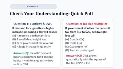
• If demand for cigarettes is highly inelastic, imposing a tax will cause: Answer: Small deadweight loss (B)

Tax Size Multiplier

• If government doubles the per-unit tax from $10 to $20, deadweight loss will: Answer: Quadruple (C)

Master Summary: Economics of Taxation

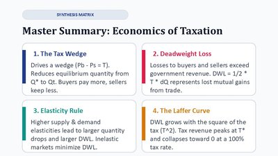
• The Tax Wedge: Drives a wedge (Pb - Ps = T), reduces equilibrium quantity, buyers pay more, sellers receive less.

• Deadweight Loss: Losses to buyers and sellers exceed government revenue; DWL = 1/2 * T * dQ.

• Elasticity Rule: Higher supply and demand elasticities lead to larger quantity drops and larger DWL; inelastic markets minimize DWL.

• The Laffer Curve: DWL grows with the square of the tax (T^2); tax revenue peaks at T* and collapses toward 0 at 100% tax rate.

Takeaways

• Taxes Are Necessary: Governments need taxes to finance public goods.

• The Economist's Goal: Design tax policies that raise required funds with minimal economic distortion (low DWL).

• Balance: Always balance efficiency (low DWL) against equity (protecting vulnerable citizens).