Motion Along a Straight Line

Introduction to 1D Kinematics

One-dimensional (1D) motion describes the movement of objects along a straight line. In this context, we analyze position, velocity, and acceleration as functions of time, focusing on cases where acceleration is constant.

• Position (x): The location of an object along a straight line.

• Velocity (v): The rate of change of position with respect to time.

• Acceleration (a): The rate of change of velocity with respect to time.

Graphs of Motion with Constant Acceleration

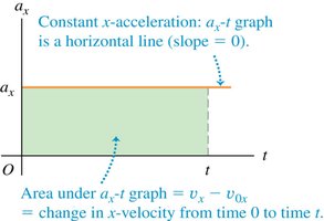
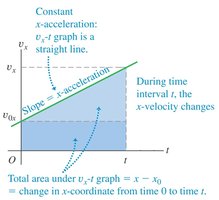
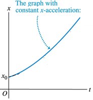
Constant acceleration leads to characteristic shapes in position-time, velocity-time, and acceleration-time graphs:

• Acceleration-Time (ax-t) Graph: A horizontal line indicates constant acceleration. The area under the curve represents the change in velocity.

• Velocity-Time (vx-t) Graph: A straight line with a slope equal to the acceleration. The area under the curve gives the change in position.

• Position-Time (x-t) Graph: A parabola, reflecting the quadratic dependence of position on time under constant acceleration.

Equations of Motion with Constant Acceleration

Kinematic Equations

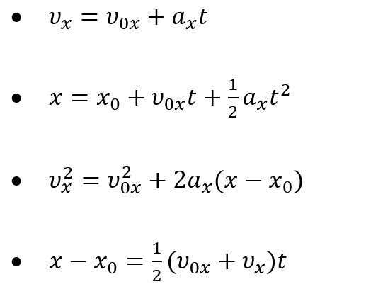
The following equations describe 1D motion with constant acceleration. They relate position, velocity, acceleration, and time, and are fundamental tools for solving kinematics problems:

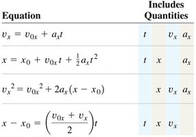
Note: Each equation is useful depending on which variables are known and which are to be found.

Worked Example: Motorcycle Acceleration

Consider a motorcycle starting at m with an initial velocity m/s and a constant acceleration m/s2. Find its velocity and position after s.

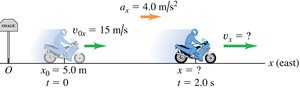
• Solution: Use the kinematic equations to solve for and .

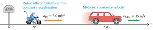
Worked Example: Police Chase

A police officer starts from rest and accelerates at m/s2 to catch a motorist moving at a constant velocity m/s. This scenario illustrates the application of kinematic equations to relative motion.

Free Fall Motion

Definition and Characteristics

Free fall refers to the motion of an object under the influence of gravity alone, with air resistance neglected. The acceleration due to gravity is denoted by and has a magnitude of m/s2, always directed downward.

• Dropped object: Initial velocity

• Thrown downward: is negative

• Thrown upward: is positive

Visualizing Free Fall

Successive images of a falling ball, taken at equal time intervals, show increasing distances between positions, indicating constant acceleration.

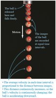
• Average velocity: Proportional to the distance between images.

• Average acceleration: Constant, equal to .

Key Points in Free Fall

• The acceleration is always (downward), regardless of the object's initial motion.

• At the highest point of upward motion, the velocity is zero, but the acceleration remains .

Graphical Analysis of Free Fall

Position-time and velocity-time graphs for free fall show the curvature and slope associated with constant negative acceleration.

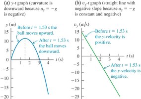
Worked Example: Ball Thrown Upward from a Roof

A ball is thrown upward with m/s from a roof. Find its position and velocity at s and s, its velocity when it is 5.00 m above the roof, the maximum height reached, and its acceleration at the maximum height.

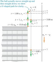
• Solution: Apply the kinematic equations for each part, noting the sign convention for upward and downward motion.

Worked Example: Dropping an Object from a Height

A one-dirham coin is dropped from the Pisa Tower and falls freely from rest. After 2.0 s, calculate its position and velocity using the kinematic equations with .

Complex Application: Predicting Impact Location

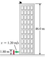
Suppose you wish to drop an egg from a 46.0 m tall building onto a moving target (professor walking at 1.20 m/s, height 1.80 m). Calculate how far from the building the professor should be when you release the egg, assuming free fall.

Summary of Kinematic Equations

The following equations are essential for solving 1D motion with constant acceleration:

Key Takeaways

• Apply kinematic equations to solve problems involving 1D motion with constant acceleration.

• Recognize free fall as a special case of 1D motion with constant downward acceleration ().

• Understand the graphical representation of position, velocity, and acceleration for constant acceleration motion.

• Be able to analyze and solve real-world problems involving free fall and projectile motion in one dimension.