Motion Along a Straight Line

Introduction to Kinematics

Kinematics is the branch of physics that describes the motion of objects without considering the causes of motion. In this chapter, we focus on motion along a straight line (one-dimensional motion), introducing key concepts such as displacement, velocity, and acceleration. These concepts are foundational for understanding more complex motions in physics.

Displacement, Time, and Average Velocity

Displacement is the change in position of a particle along a straight line, typically the x-axis. The average velocity describes how fast and in what direction the position changes over a time interval.

• Displacement (\( \Delta x \)): The difference between the final and initial positions: \( \Delta x = x_2 - x_1 \).

• Average Velocity (\( v_{\text{avg}} \)): The displacement divided by the time interval:

• Units: The SI unit for velocity is meters per second (m/s).

• Direction: Velocity is a vector; its sign indicates direction along the axis.

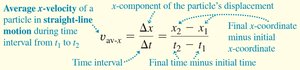
Rules for the Sign of X-Velocity

The sign of velocity indicates direction. Positive velocity means motion in the positive x-direction, while negative velocity means motion in the negative x-direction. Zero velocity means the object is momentarily at rest.

Average Velocity in Context

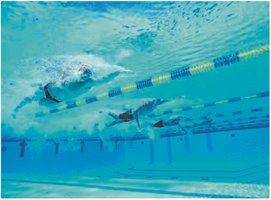
In competitive scenarios, such as a swimming race, the winner is the one with the greatest magnitude of average velocity, meaning the largest displacement in the shortest time.

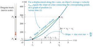
Position-Time Graphs

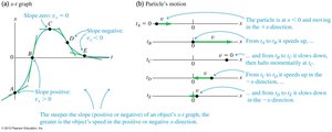
A position-time (x-t) graph visually represents how an object's position changes over time. The slope of the line on this graph corresponds to the object's velocity.

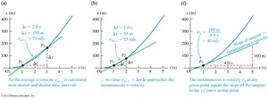
Instantaneous Velocity

Instantaneous velocity is the velocity of an object at a specific instant. It is defined as the limit of the average velocity as the time interval approaches zero:

• Instantaneous Velocity (\( v_x \)):

• It represents the slope of the tangent to the x-t curve at a given point.

Finding Velocity on an X-T Graph

To find the instantaneous velocity at a point on a position-time graph, draw a tangent to the curve at that point. The slope of this tangent line gives the instantaneous velocity.

Motion Diagrams

Motion diagrams show the position of a particle at various instants, with arrows representing velocity at each instant. They help visualize how velocity changes over time.

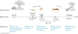
Worked Example: Cheetah Chase

Example: A cheetah starts 20 m east of a vehicle and runs toward an antelope 50 m away. Its position as a function of time is given by \( x = 20\,\text{m} + (5.0\,\text{m/s}^2)t^2 \). Tasks include finding displacement, average velocity, and instantaneous velocity at specific times.

Acceleration

Average Acceleration

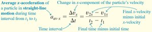
Acceleration measures how quickly velocity changes with time. The average acceleration is defined as:

• Average Acceleration (\( a_{\text{avg-x}} \)):

Instantaneous Acceleration

Instantaneous acceleration is the rate of change of velocity at a specific instant:

• Instantaneous Acceleration (\( a_x \)):

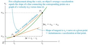
Finding Acceleration on a Vx-T Graph

On a velocity-time (vx-t) graph, the slope of the line connecting two points gives the average acceleration, while the slope of the tangent at a point gives the instantaneous acceleration.

Motion Diagrams and Acceleration

Motion diagrams can also illustrate acceleration, showing how velocity vectors change in magnitude and direction over time.

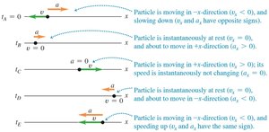
Motion with Constant Acceleration

Constant Acceleration

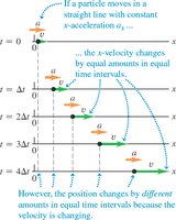
When acceleration is constant, the velocity changes by equal amounts in equal time intervals, but the position changes by different amounts due to the changing velocity.

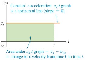
Equations of Motion with Constant Acceleration

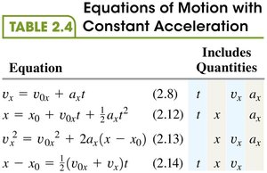
The following equations describe straight-line motion with constant acceleration:

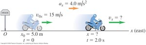
Worked Example: Motorcyclist with Constant Acceleration

Example: A motorcyclist accelerates at 4.0 m/s2 from an initial velocity of 15 m/s, starting 5.0 m east of a signpost. Find position and velocity after 2.0 s, and the position when speed is 25 m/s.

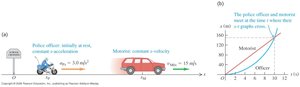
Worked Example: Police Officer in Pursuit

Example: A motorist passes a school crossing at 15 m/s. A police officer starts pursuit with constant acceleration of 3.0 m/s2. Find the time when the officer catches up, the officer's speed at that time, and the distance traveled by both vehicles.

Freely Falling Objects

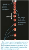
Free Fall

Free fall describes the motion of objects under the influence of gravity alone, with negligible air resistance. All objects in free fall near Earth's surface experience the same constant acceleration downward, denoted by \( g \):

• Acceleration due to gravity: (downward)

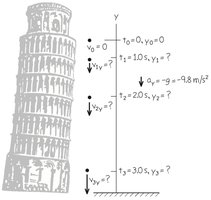
Worked Example: Coin Dropped from Leaning Tower of Pisa

Example: A coin is dropped from rest. Find its position and velocity after 1.0 s, 2.0 s, and 3.0 s, using the equations of motion for constant acceleration.

Up-And-Down Motion in Free Fall

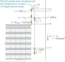
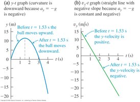
When an object is thrown vertically upward, it slows down under gravity, stops momentarily at its highest point, and then accelerates downward. The acceleration is always directed downward and has magnitude \( g \), even at the highest point where velocity is zero.

Velocity and Position by Integration

Non-Constant Acceleration

When acceleration is not constant, the equations of motion must be derived using calculus. The velocity is found by integrating acceleration over time, and position is found by integrating velocity.

• Velocity from acceleration:

• Position from velocity:

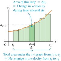
Additional info: For non-constant acceleration, graphical and numerical methods are often used to estimate position and velocity, as analytic solutions may not be possible.