One-Dimensional Kinematics

Introduction to Motion with Constant Acceleration

One-dimensional kinematics studies the motion of objects along a straight line. When acceleration is constant, the equations of motion become especially useful for predicting future positions and velocities. These equations are foundational for understanding more complex motion in physics.

Key Definitions

• Displacement (x): The change in position of an object.

• Velocity (v): The rate of change of displacement with respect to time.

• Acceleration (a): The rate of change of velocity with respect to time.

• Initial velocity (v_0): The velocity at the start of the time interval (t = 0).

• Final velocity (v): The velocity at the end of the time interval (t).

Constant Acceleration Equations of Motion

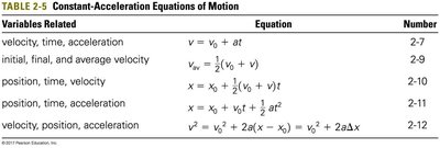
For motion with constant acceleration, the following equations relate displacement, velocity, acceleration, and time. These equations are derived from the definitions of velocity and acceleration and are essential tools for solving kinematics problems.

Graphical Interpretation of Motion

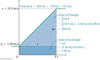
Graphs are powerful tools for visualizing motion. The area under a velocity versus time graph represents the displacement of an object. For constant acceleration, the velocity-time graph is a straight line, and the area under the curve can be calculated as the sum of a rectangle and a triangle.

Worked Examples

Example 1: Car Accelerating East and West

• A car travels east at 23.0 m/s. Find its velocity after 6.00 s if the acceleration is (a) 1.50 m/s2 east, (b) 2.5 m/s2 west.

• Use with m/s, s.

• (a) m/s$

• (b) m/s$

Example 2: Boat Accelerating from Rest

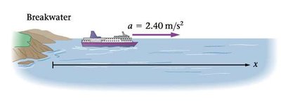
• A boat moves at 1.50 m/s, then accelerates at 2.40 m/s2 for 5.00 s after passing the breakwater.

• (a) Final velocity: m/s$

• (b) Displacement: m$

Example 3: Area Under Velocity-Time Curve

• The distance traveled by the boat in Example 2 can be found by calculating the area under the velocity-time graph.

• Area = Area of rectangle + Area of triangle = m + m = m

• This confirms the result from the kinematic equation.

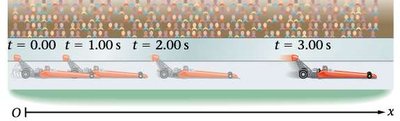
Example 4: Drag Racer's Position Over Time

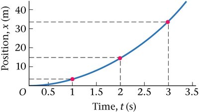
• A drag racer starts from rest and accelerates at 7.40 m/s2. Find the distance traveled after 1.00 s, 2.00 s, and 3.00 s.

• Use with , .

• (a) m

• (b) m

• (c) m

Example 5: Police Car Chasing a Speeder

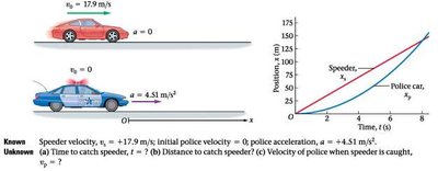
• A speeder travels at 17.9 m/s. A police car starts from rest and accelerates at 4.51 m/s2 to catch the speeder.

• Set up equations for both vehicles and solve for the time when their positions are equal.

• Speeder:

• Police:

• Set and solve for :

• s

• Distance: m

• Police velocity: m/s

Summary Table: Constant-Acceleration Equations

The following table summarizes the five key equations for one-dimensional motion with constant acceleration:

Key Takeaways

• For constant acceleration, the average acceleration equals the instantaneous acceleration.

• The area under a velocity-time graph gives the displacement.

• Choosing an appropriate coordinate system simplifies problem-solving.

• All equations are interrelated and can be derived from the definitions of velocity and acceleration.