Value of Money and the IS-LM Model

Quantity Theory of Money

The Quantity Theory of Money explains the relationship between the money supply in an economy and the general price level of goods and services. It is often summarized by the equation of exchange:

• Equation of Exchange: Where: = Money supply = Velocity of money = Price level = Real output (income)

• Implication: If the velocity of money and real output are constant, changes in the money supply directly affect the price level.

Cash Transactions Approach: Focuses on money used for transactions in the economy. Cambridge Cash Balances Approach: Emphasizes the demand for holding money as a store of value.

IS-LM Analysis

Goods Market and the IS Curve

The IS curve (Investment-Savings curve) represents equilibrium in the goods market, where aggregate demand equals aggregate output (income). It shows combinations of interest rates and income where the goods market is in equilibrium.

• Derivation of IS Curve: The IS curve is derived from the equilibrium condition , where aggregate demand equals output. Savings () must equal investment ().

• Shifts in the IS Curve:

  • Increase in government spending or autonomous investment shifts IS right.

  • Increase in taxes shifts IS left.

  • Changes in net exports, consumer confidence, or wealth can also shift the IS curve.

Money Market and the LM Curve

The LM curve (Liquidity preference-Money supply curve) represents equilibrium in the money market, where the demand for money equals the supply of money. It shows combinations of interest rates and income where the money market is in equilibrium.

• Derivation of LM Curve: The LM curve is derived from the equilibrium condition , where is the demand for money, is income, is the interest rate, is the nominal money supply, and is the price level.

• Shifts in the LM Curve:

  • Increase in money supply shifts LM right.

  • Increase in price level shifts LM left.

  • Changes in money demand due to financial innovation or expectations can shift the LM curve.

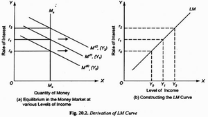
Fig. 20.2 illustrates the derivation of the LM curve. The left panel shows equilibrium in the money market at various income levels, while the right panel constructs the LM curve by plotting these equilibrium points.

Simultaneous Equilibrium in Goods and Money Markets

Equilibrium in both the goods and money markets occurs at the intersection of the IS and LM curves. This determines the equilibrium levels of income and interest rates in the economy.

• Numerical Problems: Solving for equilibrium involves finding the intersection point where both the IS and LM equations are satisfied.

Impact of Monetary and Fiscal Policy on IS-LM Model

• Monetary Policy: Changes in the money supply shift the LM curve. Expansionary policy (increasing money supply) shifts LM right, lowering interest rates and increasing income.

• Fiscal Policy: Changes in government spending or taxes shift the IS curve. Expansionary policy (increasing spending or cutting taxes) shifts IS right, raising income and interest rates.

Factors Affecting the IS Curve

• Autonomous Consumption: Higher autonomous consumption shifts IS right.

• Investment: More sensitive investment to interest rates makes IS flatter; higher autonomous investment shifts IS right.

• Government Spending: Higher spending shifts IS right.

• Taxes: Higher taxes shift IS left; lower taxes shift IS right.

• Net Exports: Higher net exports shift IS right.

• Marginal Propensity to Consume (MPC): Higher MPC makes IS steeper.

• Expectations, Technology, Wealth, Financial Conditions: Positive changes shift IS right; negative changes shift IS left.

Factors Affecting the LM Curve

• Money Supply: Higher money supply shifts LM right.

• Money Demand: Higher income increases transaction demand for money, shifting LM up.

• Interest Rate Sensitivity: High sensitivity makes LM flatter.

• Central Bank Policies: Affect money supply and LM position.

• Price Level: Higher prices shift LM left.

• Financial Innovation: Can shift LM right if money demand falls.

Laffer Curve

Meaning and Diagram

The Laffer Curve illustrates the relationship between tax rates and total tax revenue. It suggests that there is an optimal tax rate (T*) that maximizes revenue. Both very low and very high tax rates can result in low revenue.

• At 0% tax, revenue is zero; at 100% tax, revenue is also zero due to lack of incentive to work.

• Tax revenue increases with tax rate up to T*, then decreases beyond that point.

Effects of Tax Cuts

• Arithmetic Effect: Immediate reduction in revenue from lower tax rates.

• Economic Effect: Potential increase in income and spending, which can offset revenue loss.

Importance and Criticism

• Suggests governments should not always aim for the highest possible tax rate.

• Used as a basis for tax cuts in the 1980s (e.g., Reagan Administration).

• Criticized for oversimplifying tax systems and not accounting for all economic complexities.

Supply-Side Economics

Meaning and Principles

Supply-side economics focuses on increasing production and aggregate supply to drive long-term economic growth. It emphasizes reducing barriers to production, such as taxes and regulations.

• Associated with Say's Law: "Supply creates its own demand." Production generates income, which enables consumption.

Major Policy Measures

• Tax Cuts: Encourage work, saving, and investment.

• Deregulation: Reduces business costs and encourages competition.

• Privatization: Transfers state assets to private sector for efficiency.

• Investment in Human Capital and Infrastructure: Improves productivity and capacity.

• Trade Liberalization and Lower Borrowing Costs: Encourages investment and competitiveness.

Supply-Side vs Demand-Side Economics

• Supply-side: Focuses on long-run growth by increasing productive capacity.

• Demand-side (Keynesian): Focuses on short-run stabilization by increasing aggregate demand.

Conclusion

Supply-side economics aims for long-term growth through policies that enhance production, such as tax cuts, deregulation, privatization, and investment in human capital and infrastructure.