 Indietro
Chapter 3: Numerically Summarizing Data – Introductory Statistics Study Guide
Guida di studio - Note intelligenti
 Appunti personalizzati basati sui tuoi materiali, ampliati con definizioni chiave, esempi e contesto.
Chapter 3: Numerically Summarizing Data
3.1 Measures of Central Tendency
Measures of central tendency are statistical values that describe the center of a data set. The most common measures are the mean, median, and mode. Each provides a different perspective on the data's central value.
3.1.1 Arithmetic Mean
The arithmetic mean is the sum of all values divided by the number of observations. It is commonly referred to as the "average." The mean can be calculated for both populations and samples.
Population Mean (μ): Uses all individuals in the population. It is a parameter.
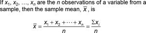
Sample Mean (\(\bar{x}\)): Uses a subset (sample) of the population. It is a statistic.
Formula for Sample Mean:
Formula for Population Mean:
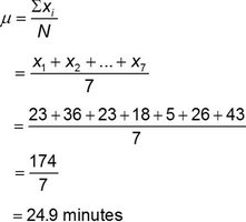
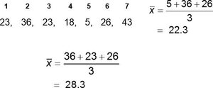
Example: Travel times to work for seven employees: 23, 36, 23, 18, 5, 26, 43. Population mean: minutes.
3.1.2 Median
The median is the value in the middle of a data set when arranged in ascending order. It divides the data into two equal halves.
Finding the Median:
Step 1: Arrange data in ascending order.
Step 2: Determine the number of observations, n.
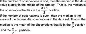
Step 3: If n is odd, the median is the value at position . If n is even, the median is the mean of the values at positions and .
Example (Odd n): Data: 5, 18, 23, 23, 26, 36, 43. Median is 23.

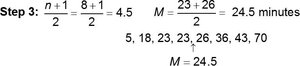
Example (Even n): Data: 5, 18, 23, 23, 26, 36, 43, 70. Median is minutes.
3.1.3 Resistance of Statistics
A statistic is resistant if it is not substantially affected by extreme values (outliers). The median is resistant, while the mean is not.
Example: Adding a new employee with a 130-minute commute increases the mean more than the median.
Mean before: 24.9 minutes; Median before: 23 minutes
Mean after: 38 minutes; Median after: 24.5 minutes
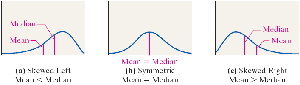
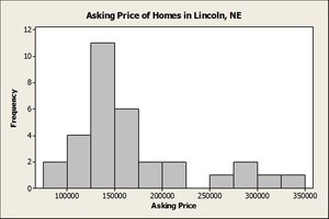
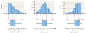
Distribution Shape: If mean > median, distribution is skewed right; if mean < median, skewed left; if mean ≈ median, symmetric.
3.1.4 Mode
The mode is the most frequent value in a data set. A set can have no mode, one mode, or multiple modes.
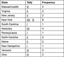
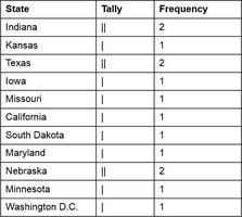
Example: Mode of Vice Presidents' state of birth.
State | Tally | Frequency |
|---|---|---|
New York | |||| |||| | 8 |
Massachusetts | ||| | 3 |
Virginia | || | 2 |
New Jersey | || | 2 |
South Carolina | | | 1 |
Kentucky | |||| | 4 |
Pennsylvania | | | 1 |
North Carolina | || | 2 |
Maine | | | 1 |
New Hampshire | | | 1 |
Vermont | ||| | 3 |
Ohio | ||| | 3 |
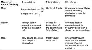
Comparison Table: Measures of Central Tendency
Measure | Computation | Interpretation | When to Use |
|---|---|---|---|
Mean | Population: Sample: | Center of Gravity | Quantitative, symmetric distribution |
Median | Arrange data, divide in half | Divides bottom 50% from top 50% | Quantitative, skewed distribution |
Mode | Tally most frequent | Most frequent observation | Qualitative or when most frequent is desired |
3.2 Measures of Dispersion
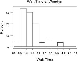
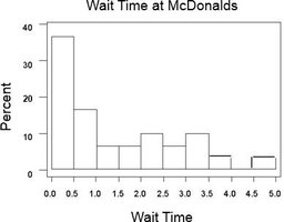
Measures of dispersion describe the spread or variability of a data set. Common measures include range, variance, and standard deviation.
3.2.1 Range
The range is the difference between the largest and smallest values.
Formula:
Example: Data: 23, 36, 23, 18, 5, 26, 43. Range: minutes.
3.2.2 Standard Deviation
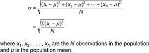
The standard deviation measures the average distance of data values from the mean. It is calculated differently for populations and samples.
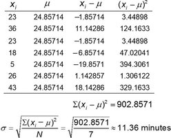
Population Standard Deviation (σ):
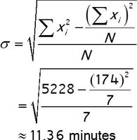
Computational formula:
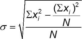
Example: Data: 23, 36, 23, 18, 5, 26, 43. minutes.
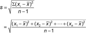
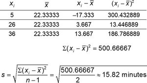
Sample Standard Deviation (s):
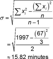
Computational formula:
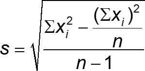
Example: Sample: 5, 26, 36. minutes.
3.2.3 Variance
The variance is the square of the standard deviation. Population variance is , sample variance is .
Example: Population variance: minutes; Sample variance: minutes.
3.2.4 Empirical Rule
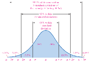
The Empirical Rule applies to bell-shaped (normal) distributions:
68% of data within 1 standard deviation of mean
95% within 2 standard deviations
99.7% within 3 standard deviations
3.2.5 Chebyshev’s Inequality
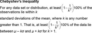
Chebyshev’s Inequality applies to any data set, regardless of shape. For any k > 1:
At least of the data lies within k standard deviations of the mean.

3.3 Measures from Grouped Data
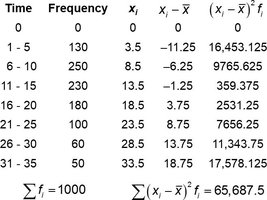
When data is grouped in frequency distributions, we can approximate central tendency and dispersion.
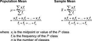
3.3.1 Approximate Mean from Grouped Data
Use class midpoints and frequencies:
3.3.2 Weighted Mean
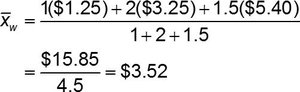
The weighted mean accounts for values with different weights:
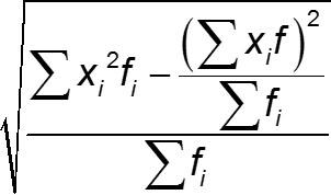
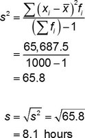
3.3.3 Approximate Standard Deviation from Grouped Data
Use class midpoints and frequencies:
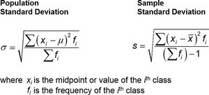
Computational formula:
3.4 Measures of Position and Outliers
Measures of position describe the relative standing of a data value within a data set.
3.4.1 z-Scores
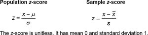
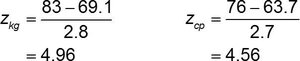
A z-score measures how many standard deviations a value is from the mean.
Population: Sample:
Example: Comparing heights using z-scores.
3.4.2 Percentiles
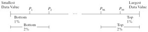
The kth percentile is the value below which k percent of the data falls.
3.4.3 Quartiles
Quartiles divide data into four equal parts:
Q1: 25th percentile
Q2: 50th percentile (median)
Q3: 75th percentile

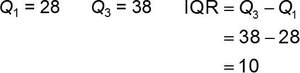
3.4.4 Interquartile Range (IQR)
The interquartile range is the range of the middle 50% of data:
3.4.5 Outliers
Outliers are values that fall outside the "fences" defined by quartiles and IQR:
Lower Fence:
Upper Fence:
Values outside these fences are considered outliers.
3.5 Five-Number Summary and Boxplots
The five-number summary consists of: minimum, Q1, median, Q3, maximum. Boxplots visually display this summary and help identify outliers and distribution shape.
3.5.1 Five-Number Summary
Minimum
Q1
Median (Q2)
Q3
Maximum
3.5.2 Boxplots
Boxplots are graphical representations of the five-number summary. They show the spread, center, and outliers of a data set.

Additional info: This study guide covers all major concepts from Chapter 3, including formulas, examples, and visual aids for central tendency, dispersion, position, and graphical summaries. It is suitable for exam preparation in an Introductory Statistics course.
