Density Curves

Definition and Properties

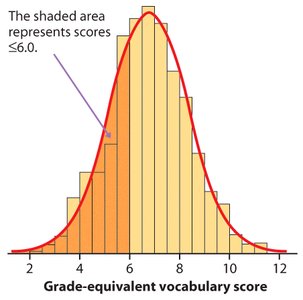
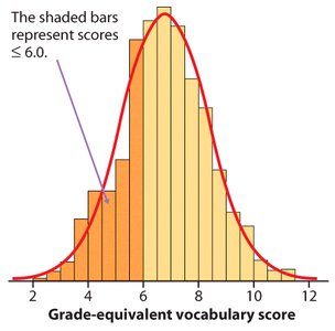
A density curve is a mathematical model used to describe the distribution of a variable. The total area under the curve is always equal to 1, representing 100% of the data. The area under the curve within a specific interval corresponds to the proportion or percentage of individuals whose values fall within that interval.

• Key Point 1: Density curves can take any shape, depending on the distribution of the data.

• Key Point 2: Some density curves are well-known mathematically, such as the normal curve, while others are not.

• Example: The shaded area under a density curve can represent the proportion of students scoring below a certain grade-equivalent vocabulary score.

Median and Mean of a Density Curve

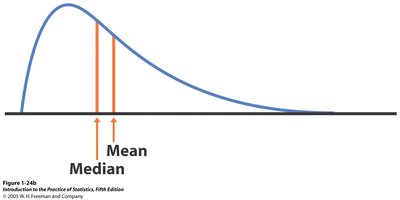
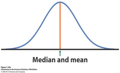
The median of a density curve is the point that divides the area under the curve into two equal halves. The mean is the balance point of the curve, where it would balance if made of solid material. For symmetric density curves, the mean and median are the same. For skewed curves, the mean is pulled in the direction of the longer tail.

• Key Point 1: In symmetric distributions, mean = median.

• Key Point 2: In skewed distributions, the mean is affected by the skewness.

• Example: Income distributions are often skewed, with the mean higher than the median.

The Normal Distribution

Characteristics and Mathematical Model

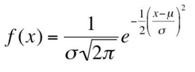
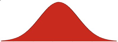
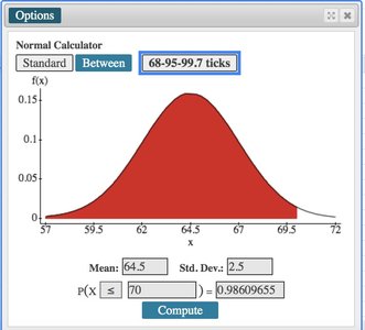
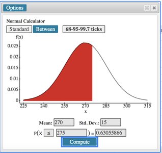
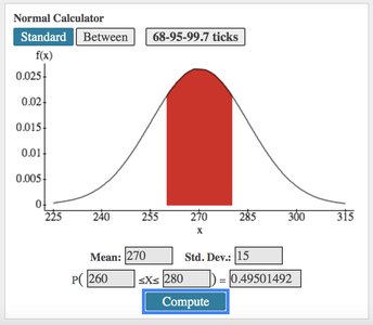
The normal distribution is a family of symmetrical, bell-shaped density curves defined by a mean (\(\mu\)) and a standard deviation (\(\sigma\)). It is also known as the Gaussian distribution. The normal model is denoted as N(\(\mu\), \(\sigma\)).

• Key Point 1: The normal distribution is unimodal and symmetric.

• Key Point 2: Most values cluster around the mean, with fewer values farther from the center.

• Formula: The probability density function for the normal distribution is:

• Example: Heights, test scores, and measurement errors often follow a normal distribution.

Normal Distribution Parameters

• \(\mu\) (mu): Population mean

• \(\sigma\) (sigma): Population standard deviation

• N(\(\mu\), \(\sigma\)): Normal model with specified mean and standard deviation

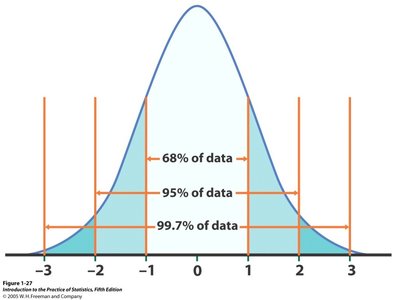
Empirical Rule (68-95-99.7% Rule)

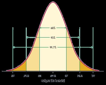
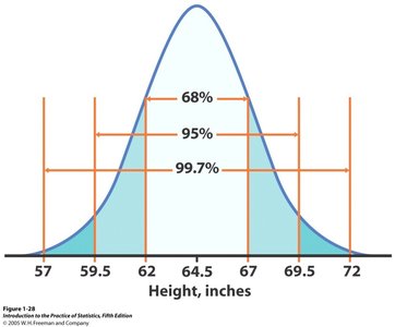
The Empirical Rule describes the spread of data in a normal distribution:

• About 68% of observations are within 1 standard deviation of the mean.

• About 95% are within 2 standard deviations.

• About 99.7% are within 3 standard deviations.

Standardization and Z-Scores

Definition and Calculation

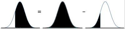
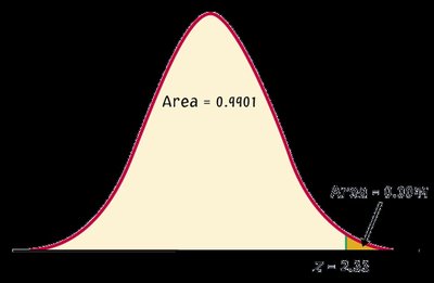
A z-score measures how many standard deviations a data value is from the mean. Standardizing transforms any normal distribution N(\(\mu\), \(\sigma\)) into the standard normal distribution N(0,1).

• Formula:

• Key Point 1: Positive z-scores indicate values above the mean; negative z-scores indicate values below the mean.

• Key Point 2: Z-scores allow comparison across different normal distributions.

• Example: An exam score of 88 with mean 83 and standard deviation 5:

Interpretation of Z-Scores

• Small z-score: Value is close to the mean.

• Large z-score: Value is far from the mean.

• Example: For height, a z-score of -0.6 means the value is below the mean but not extreme; a z-score of +2.2 is above the mean and considered extreme.

Checking for Normality

Assumptions and Conditions

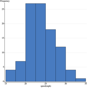
Before applying the normal model, it is important to check whether the data meet the Nearly Normal Condition:

• Key Point 1: The sample should be representative, symmetric, unimodal, and have no major outliers.

• Key Point 2: Use histograms and QQ plots to assess normality.

• Example: QQ plots compare sample data to expected z-scores; if points follow the diagonal, the distribution is approximately normal.

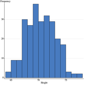
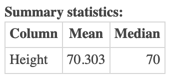
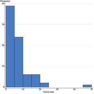
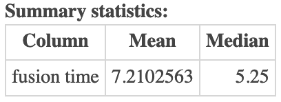
Summary Table: Mean and Median Comparison

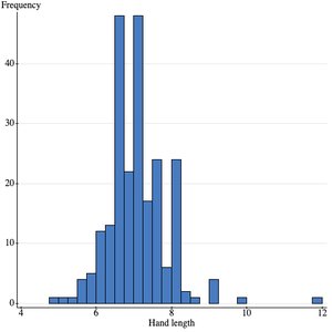
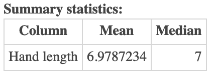
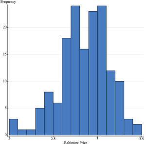
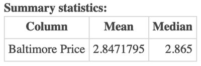
The following table summarizes the mean and median for several sample distributions, illustrating the relationship between these measures in symmetric and skewed distributions.

Additional info: The notes above expand on the original content by providing definitions, formulas, and examples for density curves, normal distributions, z-scores, and checking for normality, ensuring completeness and academic quality for introductory statistics students.