Chapter 4: Describing the Relation Between Two Variables

4.1 Scatter Diagrams and Correlation

This section explores how to visually and numerically describe the relationship between two quantitative variables. The main tools are scatter diagrams and the linear correlation coefficient.

4.1.1 Draw and Interpret Scatter Diagrams

• Response Variable (y): The variable whose value is explained or predicted by the explanatory variable.

• Explanatory Variable (x): The variable that explains changes in the response variable.

• Scatter Diagram: A graph showing the relationship between two quantitative variables for the same individual. Each point represents one individual’s values for both variables. The explanatory variable is plotted on the horizontal axis, and the response variable on the vertical axis.

• Types of Relationships: Scatter diagrams can reveal linear, nonlinear, or no relationship between variables.

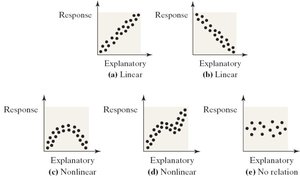
• Positive Association: As one variable increases, the other also increases.

• Negative Association: As one variable increases, the other decreases.

4.1.2 Properties of the Linear Correlation Coefficient

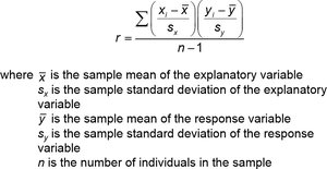
The linear correlation coefficient (Pearson’s r) measures the strength and direction of the linear relationship between two quantitative variables.

• Population correlation coefficient: (rho)

• Sample correlation coefficient:

• Formula for r:

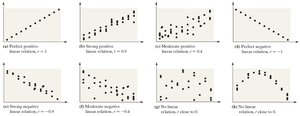
• Properties:

  • indicates a perfect positive linear relation.

  • indicates a perfect negative linear relation.

  • The closer is to +1 or -1, the stronger the linear relationship.

  • If is close to 0, there is little or no linear relationship.

  • is unitless and not resistant to outliers.

4.1.3 Compute and Interpret the Linear Correlation Coefficient

To compute , use the formula above with the data values. Interpretation involves both the sign (direction) and the magnitude (strength) of .

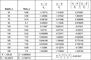
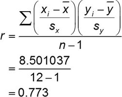
• Example: For drilling data, indicates a strong positive linear relationship between drilling depth and time to drill five feet.

4.1.4 Determine Whether a Linear Relation Exists

To test for a linear relationship:

1. Calculate the absolute value of .

2. Find the critical value for the sample size (from statistical tables).

3. If is greater than the critical value, a linear relation exists.

• Example: For , critical value = 0.576. Since , a positive linear relation exists.

4.1.5 Correlation vs. Causation

• Correlation does not imply causation. A high correlation between two variables does not mean that one causes the other.

• Lurking Variable: A variable not included in the study that affects both the explanatory and response variables, possibly creating a spurious association.

• Example: Ice cream sales and crime rates are correlated due to the lurking variable of temperature.

• Observational vs. Experimental Data: Only experiments can establish causality; observational studies can only show association.

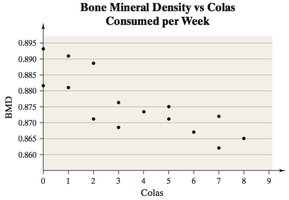
• Example: In a study of cola consumption and bone mineral density, a negative correlation was found, but lurking variables (e.g., BMI, calcium intake) prevent a causal conclusion.

4.2 Least-Squares Regression

This section introduces the least-squares regression line, which models the linear relationship between two variables and allows for prediction.

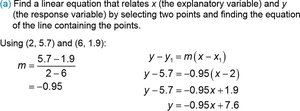
4.2.1 Find the Least-Squares Regression Line and Use the Line to Make Predictions

• Least-Squares Regression Line: The line that minimizes the sum of squared residuals (errors) between observed and predicted values.

• Residual: The difference between the observed value and the predicted value:

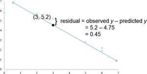
• Least-Squares Criterion: Minimize

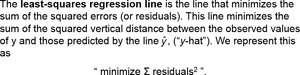
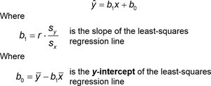
• Equation of the Least-Squares Regression Line:

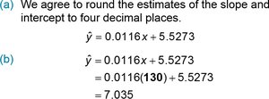
• Example: For drilling data,

• To predict time at feet: minutes

4.2.2 Interpret the Slope and y-Intercept

• Slope (): The change in the response variable for each unit increase in the explanatory variable. For the drilling example, each additional foot increases drilling time by 0.0116 minutes, on average.

• y-Intercept (): The predicted value of y when x = 0. For the drilling example, starting at the surface (x = 0), the predicted time is 5.5273 minutes.

• Scope of the Model: Predictions should only be made within the range of observed x-values.

4.2.3 Compute the Sum of Squared Residuals

• The least-squares regression line always has the smallest possible sum of squared residuals compared to any other line.

4.3 Diagnostics on the Least-Squares Regression Line

This section discusses how to assess the fit of the regression line using the coefficient of determination.

4.3.1 Compute and Interpret the Coefficient of Determination ()

• Coefficient of Determination (): Measures the proportion of total variation in the response variable explained by the regression line.

• If , the line explains none of the variation; if , it explains all the variation.

• Calculation: for simple linear regression.

• Example: For drilling data, , so (59.75% of the variability in drilling time is explained by depth).

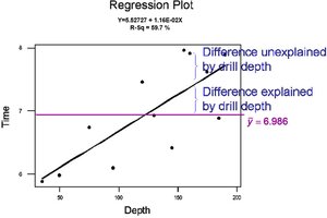
• Deviations:

  • Total deviation:

  • Explained deviation:

  • Unexplained deviation:

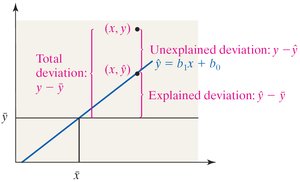
• Relationship: Total Deviation = Explained Deviation + Unexplained Deviation

• Variation: Total Variation = Explained Variation + Unexplained Variation

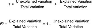
• Formula for :

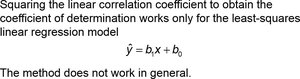
• Comparing Data Sets: can be used to compare how well the regression line fits different data sets.

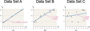
• Data Set A: 99.99% of variability explained

• Data Set B: 94.7% of variability explained

• Data Set C: 9.4% of variability explained

Additional info: These notes cover the core concepts of Chapter 4, including scatter diagrams, correlation, regression, and diagnostics, as outlined in a typical Introductory Statistics curriculum.