Ch. 2 - Descriptive Statistics

2.1 Frequency Distributions and Their Graphs

Frequency distributions are foundational tools in statistics for organizing and summarizing data. They display how data values are distributed across different intervals or classes, making it easier to interpret large data sets.

Frequency Distribution

• Definition: A table that shows classes (intervals) of data with a count of the number of entries in each class.

• Frequency (f): The number of data entries in a class.

Example Table:

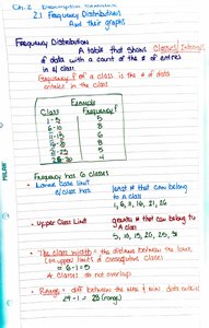
• Lower Class Limit: The smallest number that can belong to a class (e.g., 0, 6, 11, 16, 21).

• Upper Class Limit: The largest number that can belong to a class (e.g., 5, 10, 15, 20, 25).

• Class Width: The difference between the lower limits of consecutive classes.

• Class Boundaries: Numbers that separate classes without gaps. For integer data, subtract 0.5 from the lower limit and add 0.5 to the upper limit.

• Range: The difference between the maximum and minimum data values.

Guidelines for Constructing a Frequency Distribution

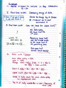
1. Decide the number of classes (commonly 5–20).

2. Find the class width: (round up to the next convenient number).

3. Find class limits and boundaries.

Types of Frequency Distributions

• Open-Ended Classes: Classes with no specific lower or upper boundary (e.g., "70 and above").

• Relative Frequency: The proportion of data that falls in a class.

• Cumulative Frequency: The sum of the frequencies for that class and all previous classes.

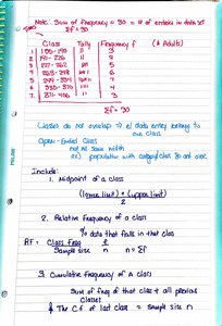
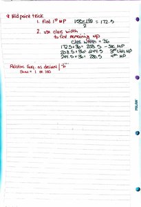
Midpoint of a Class

• Formula:

• Used for graphing and calculating the mean of grouped data.

Frequency Distribution Table Example

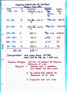
Frequency Histogram

• A bar graph that represents the frequency distribution of a data set.

• The horizontal axis shows class boundaries or midpoints; the vertical axis shows frequency.

• Bars are adjacent (no gaps) and begin/end at class boundaries.

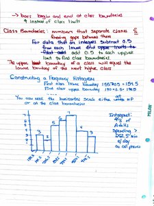
Frequency Polygon

• A line graph that emphasizes the change in frequencies.

• Plot points at the class midpoints and connect them with straight lines.

• Begin and end the graph at the midpoints of the classes just before the first and after the last class.

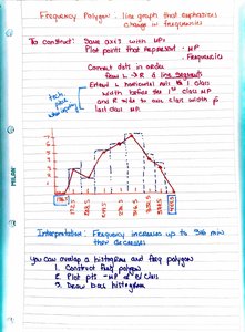
Relative Frequency Histogram

• Similar to a frequency histogram, but the vertical axis represents relative frequency instead of absolute frequency.

• Useful for comparing distributions with different sample sizes.

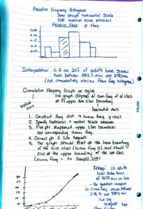
Cumulative Frequency Graph (Ogive)

• A line graph that displays the cumulative frequency of each class at its upper boundary.

• Helps determine the number of data values below a particular value.

2.2 More Graphs and Displays

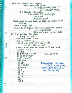
Stem-and-Leaf Plot

• Displays data by separating each value into a stem (all but the last digit) and a leaf (the last digit).

• Shows the shape of the data and retains actual data values.

• Useful for small to moderate-sized data sets.

Dot Plot

• Shows the distribution of data by plotting each data value as a dot above a number line.

• Helps identify clusters, gaps, and outliers.

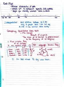
Pie Chart

• Represents qualitative data as sectors of a circle, where the area of each sector is proportional to the frequency or relative frequency.

• Useful for showing the proportion of categories in a whole.

Pareto Chart

• A bar graph for qualitative data, with bars arranged in order of decreasing frequency.

• Highlights the most significant categories.

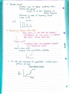
Time Series Graph

• Plots data values against time, showing trends or patterns over intervals.

• Each point represents a quantitative variable at a specific time.

2.3 Measures of Central Tendency

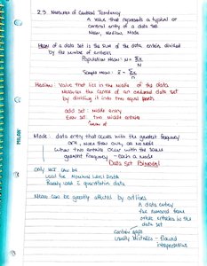
Measures of central tendency describe the center or typical value of a data set. The three main measures are the mean, median, and mode.

Mean

• Definition: The sum of all data entries divided by the number of entries.

• Population Mean:

• Sample Mean:

Median

• The middle value when the data is ordered from least to greatest.

• If the number of entries is even, the median is the mean of the two middle values.

Mode

• The data entry that occurs most frequently.

• A data set may have one mode (unimodal), more than one mode (bimodal or multimodal), or no mode.

Mean of a Frequency Distribution

• For grouped data, the mean is calculated using class midpoints and frequencies.

• Formula: , where is the class midpoint and is the class frequency.

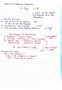
The Shapes of Distributions

• Symmetric: Both sides of the distribution are mirror images.

• Skewed Left (Negatively Skewed): The mean is less than the median.

• Skewed Right (Positively Skewed): The mean is greater than the median.

Summary: Understanding frequency distributions and their graphical representations is essential for summarizing and interpreting data in statistics. These tools provide insight into the shape, center, and spread of data sets, forming the basis for further statistical analysis.