Chapter 2: Exploring Data with Graphs and Numerical Summaries

Introduction

Descriptive statistics provide essential tools for summarizing and understanding data. Graphical summaries offer visual insights into the distribution and shape of data, while numerical summaries quantify central tendency and variability. This chapter covers the main methods for describing and interpreting quantitative data.

Describing the Center of Quantitative Data

Mean

The mean (arithmetic average) is calculated by summing all observations and dividing by the number of observations. It represents the "center of mass" of the data.

• Formula:

• All data values influence the mean.

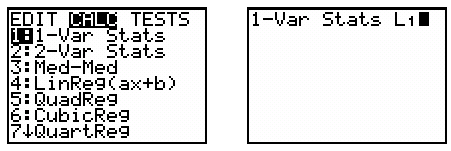
• Calculator instructions: Enter data into L1, then use STAT > CALC > 1:1-Var Stats.

Median

The median is the midpoint of the ordered data. It divides the data into two equal halves.

• If n is odd, the median is the middle value.

• If n is even, the median is the average of the two middle values.

• To find the median, sort the data and use the position formula: .

Comparing Mean and Median

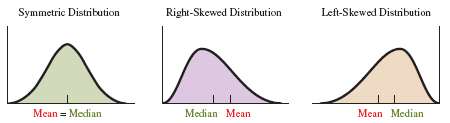
The mean and median are close in symmetric distributions. In skewed distributions, the mean is pulled toward the tail, while the median is more resistant to outliers.

• For symmetric data, use the mean.

• For skewed data, use the median.

Resistant Measures

A resistant measure is not influenced much by extreme values (outliers). The median is resistant; the mean is not.

Mode

The mode is the value that occurs most frequently in a dataset. It is most useful for categorical data and corresponds to the highest bar in a histogram.

Describing the Spread of Quantitative Data

Range

The range is the difference between the largest and smallest values in the dataset.

• Formula:

• The range is sensitive to outliers.

Standard Deviation

The standard deviation measures the average distance of data values from the mean. It is calculated as the square root of the variance.

• Formula:

• Standard deviation has the same units as the data.

• Variance () is the squared standard deviation.

• Not resistant to outliers.

Empirical Rule

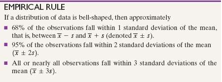
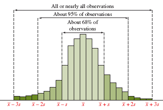
For bell-shaped (normal) distributions:

• About 68% of data falls within 1 standard deviation of the mean ().

• About 95% falls within 2 standard deviations ().

• Nearly all falls within 3 standard deviations ().

Measures of Position and Spread

Percentiles

The pth percentile is the value below which p% of the observations fall.

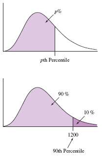
Quartiles and the Five-Number Summary

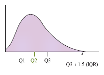
Quartiles divide ordered data into four equal parts:

• Q1: First quartile (25th percentile)

• Q2: Second quartile (median, 50th percentile)

• Q3: Third quartile (75th percentile)

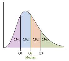
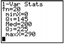
The five-number summary consists of: minimum, Q1, median, Q3, and maximum.

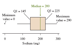
Interquartile Range (IQR) and Outliers

The interquartile range (IQR) measures the spread of the middle 50% of data:

• Formula:

• Potential outlier: Any value < or >

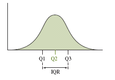
Boxplots

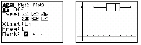
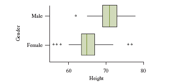
Boxplots visually display the five-number summary and highlight potential outliers. They are useful for comparing distributions but do not show the shape as clearly as histograms.

Comparing Distributions

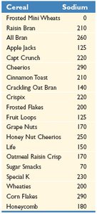
Boxplots are effective for comparing the spread and center of two or more distributions, especially when examining differences between groups.

Z-Score

The z-score indicates how many standard deviations an observation is from the mean:

• Formula:

• Observations with are considered potential outliers in bell-shaped distributions.

Constructing and Interpreting Graphs

Guidelines for Effective Graphs

• Label both axes and provide clear headings.

• Start the vertical axis at zero for accurate comparisons.

• Use appropriate graph types (bars, lines, points).

• Be cautious when comparing groups with different scales.

Misuse of Graphical Summaries

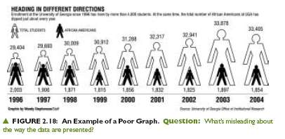
Poorly constructed graphs can mislead viewers. Always check for accurate scaling, labeling, and representation of data.

Summary Table: Measures of Center and Spread

Summary

• Use mean and standard deviation for symmetric data without outliers.

• Use the five-number summary and IQR for skewed data or when outliers are present.

• Graphical and numerical summaries together provide a comprehensive understanding of data.