Exploring Data with Tables and Graphs

Overview

This section introduces various graphical methods for organizing, summarizing, and interpreting data in statistics. Understanding these visual tools is essential for accurately describing data distributions and avoiding misleading representations.

Graphs that Enlighten

Dotplots

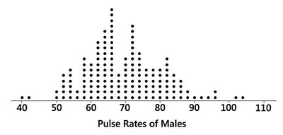
Dotplots are simple graphs used to display quantitative data. Each data value is represented as a dot above a horizontal scale, and dots representing equal values are stacked vertically. Dotplots are useful for visualizing the shape of a distribution and can often allow reconstruction of the original data set.

• Displays the shape of the data distribution.

• Retains original data values, making it possible to recreate the data set.

Example: Pulse rates of males visualized as a dotplot.

Stemplots (Stem-and-Leaf Plots)

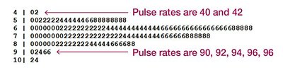
Stemplots (or stem-and-leaf plots) represent quantitative data by splitting each value into a "stem" (typically the leftmost digit) and a "leaf" (typically the rightmost digit). This method retains the original data values and sorts them, making it easy to see the distribution and order.

• Shows the shape of the distribution.

• Retains original data values.

• Data are sorted in order.

Example: Pulse rates organized in a stem-and-leaf plot.

Time-Series Graphs

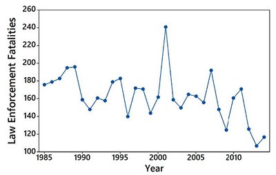
Time-series graphs display quantitative data collected at different points in time (e.g., monthly or yearly). These graphs are valuable for identifying trends and patterns over time.

• Reveals trends and changes in data over time.

Example: Law enforcement fatalities over several years.

Bar Graphs

Bar graphs use bars of equal width to show frequencies of categories in categorical (qualitative) data. Bars may be separated by gaps, and the graph makes it easy to compare different categories.

• Shows relative distribution of categorical data.

• Facilitates comparison between categories.

Pareto Charts

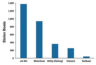
Pareto charts are specialized bar graphs for categorical data, with bars arranged in descending order of frequency. This arrangement highlights the most important categories.

• Shows relative distribution of categorical data.

• Draws attention to the most significant categories.

Example: Pareto chart of stolen boats.

Pie Charts

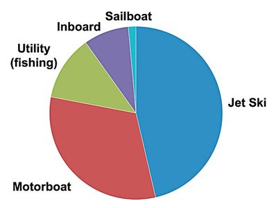
Pie charts depict categorical data as slices of a circle, with each slice proportional to the frequency of the category. This format is commonly used to show the distribution of categorical data.

• Shows distribution of categorical data in a familiar format.

Example: Pie chart of stolen boats.

Frequency Polygons

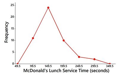
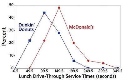
Frequency polygons use line segments connected to points above class midpoints to display frequency distributions. They are similar to histograms but use lines instead of bars. A variation is the relative frequency polygon, which uses proportions or percentages for the vertical scale.

• Visualizes frequency distributions using line segments.

• Relative frequency polygons compare distributions using percentages.

Example: Frequency polygon of McDonald's lunch service times.

Example: Relative frequency polygons comparing McDonald's and Dunkin' Donuts.

Graphs That Deceive

Nonzero Vertical Axis

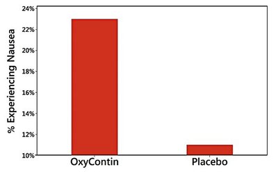
Some graphs use a vertical scale that starts at a value greater than zero, exaggerating differences between groups. Always check the axis to ensure accurate interpretation.

• Exaggerates differences by not starting the vertical axis at zero.

• Careful examination is needed to avoid misinterpretation.

Example: Comparison of bar graphs with different vertical axis starting points.

Pictographs

Pictographs use drawings of objects to represent data. When one-dimensional data are depicted with two- or three-dimensional objects, differences can be grossly distorted due to geometric scaling. For example, doubling the sides of a square increases its area by four times, and doubling the sides of a cube increases its volume by eight times.

• Can distort differences due to geometric scaling.

• Misleading visual representation of data.

Concluding Thoughts

There are many useful graphs in statistics, and new types are continually being developed. The principles of effective graph design include:

• For small data sets (20 values or fewer), use a table instead of a graph.

• A graph should focus on the true nature of the data, not on distracting design features.

• Do not distort data; construct graphs to reveal the true nature of the data.

• Most of the ink in a graph should be used for the data, not for other design elements.

Additional info: These principles are based on Edward Tufte's guidelines for the visual display of quantitative information.