Describing Data with Tables and Graphs

Frequency Distributions for Organizing and Summarizing Data

Frequency distributions are essential tools in statistics for organizing raw data into a more interpretable format. They display how data values are distributed across different intervals or categories, making it easier to identify patterns, trends, and outliers.

• Frequency Distribution: A table that divides data into classes or intervals and shows the number of data values in each class.

• Purpose: To summarize large data sets, facilitate comparison, and prepare data for graphical representation.

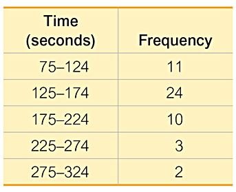
• Example: The table below shows the frequency distribution of McDonald's lunch service times.

Histograms

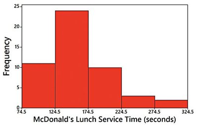
A histogram is a graphical representation of a frequency distribution. It consists of adjacent bars whose heights correspond to the frequency (or relative frequency) of data within each class interval. Histograms are particularly useful for visualizing the shape, center, and spread of quantitative data.

• Definition: A bar graph with bars of equal width, drawn adjacent to each other (unless there are gaps in the data).

• Horizontal Axis: Represents classes of quantitative data values.

• Vertical Axis: Represents frequencies or relative frequencies.

• Key Uses:

  • Displays the shape of the data distribution

  • Identifies outliers

  • Shows the spread and center of the data

• Example: The histogram below visualizes the frequency distribution of McDonald's lunch service times.

Relative Frequency Histograms

A relative frequency histogram is similar to a standard histogram, but the vertical axis represents the proportion (or percentage) of data values in each class, rather than the raw frequency. This allows for easier comparison between data sets of different sizes.

• Relative Frequency: Calculated as

• Shape and Scale: The shape and horizontal scale are identical to the frequency histogram; only the vertical scale changes.

Interpreting Histograms: The CVDOT Approach

When analyzing histograms, statisticians often use the CVDOT framework to extract meaningful information:

• Center: Where is the middle of the data?

• Variation: How spread out is the data?

• Distribution: What is the overall shape?

• Outliers: Are there any unusual values?

• Time: Is there a time component or trend?

Common Distribution Shapes

Normal (Bell-Shaped) Distribution

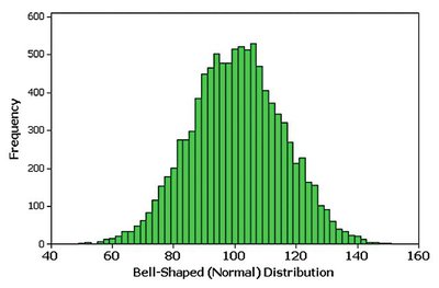
A normal distribution is symmetric and bell-shaped, with most data values clustering around the center and fewer values appearing as you move away from the center in either direction.

• Properties:

  • Symmetric about the mean

  • Mean, median, and mode are equal

  • Follows the empirical rule (68-95-99.7%)

• Example: The histogram below shows a bell-shaped (normal) distribution.

Uniform Distribution

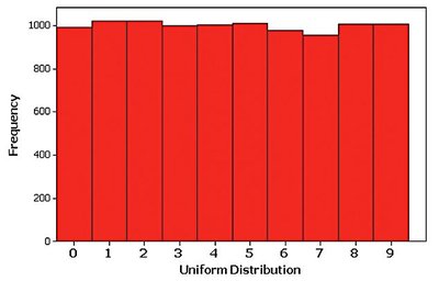
In a uniform distribution, all intervals have approximately the same frequency. The histogram appears flat, indicating that all outcomes are equally likely.

• Properties: No clear peak; frequencies are roughly equal across all classes.

• Example: The histogram below illustrates a uniform distribution.

Skewed Distributions

A distribution is skewed if it is not symmetric and extends more to one side than the other.

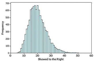
• Skewed to the Right (Positively Skewed): The right tail is longer; most data are concentrated on the left.

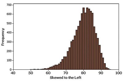
• Skewed to the Left (Negatively Skewed): The left tail is longer; most data are concentrated on the right.

• Examples: The histograms below show right and left skewness, respectively.

Assessing Normality with Normal Quantile Plots

Normal Quantile (Q-Q) Plots

Normal quantile plots (also called Q-Q plots) are graphical tools used to assess whether a data set follows a normal distribution. They plot observed data values against expected z-scores from a standard normal distribution.

• Criteria for Normality:

  • If the points are reasonably close to a straight line and do not show a systematic pattern, the data are approximately normal.

  • If the points deviate significantly from a straight line or show a systematic pattern, the data are not normal.

• Examples: The plots below illustrate normal and non-normal distributions.

Summary Table: Distribution Shapes and Their Properties

Additional info: The CVDOT framework is a common approach in introductory statistics for interpreting histograms and understanding the underlying data distribution. Normal quantile plots are also referred to as Q-Q plots in statistical literature.