 Indietro
Foundations and Exploratory Concepts in College Statistics
Guida di studio - Note intelligenti
 Appunti personalizzati basati sui tuoi materiali, ampliati con definizioni chiave, esempi e contesto.
Statistical Thinking
Overview of Statistical Processes
Statistical thinking involves understanding how data is collected, analyzed, and interpreted to draw meaningful conclusions. The process typically follows a structured approach:
Purpose: Define the goal of the statistical study.
Prepare: Consider what the data means, the context, and how it was collected.
Analyze: Explore and summarize the data using statistical methods.
Conclude: Draw conclusions based on the analysis.
Key Concepts
Population vs. Sample:
Population: The entire collection of data or subjects of interest.
Sample: A subset of the population used for analysis.
Observations: Individual data points collected in a study.
Measurements: Quantitative or qualitative values assigned to observations.
Sampling
Representativeness and Methods
Sampling is the process of selecting a subset of the population to make inferences about the whole. A representative sample closely resembles the population in relevant characteristics.
Random Sampling: Every member of the population has an equal chance of being selected.
Convenience Sampling: Choosing individuals who are easiest to reach.
Stratified Sampling: Dividing the population into subgroups and sampling from each.
Cluster Sampling: Dividing the population into clusters and randomly selecting clusters.
Exploring Data: Tables and Graphs
Frequency Distributions
Frequency distributions summarize data by showing how often each value or category occurs. They are foundational for exploratory data analysis (EDA).
Defining Categories:
Natural categories (e.g., gender, age groups).
Constructed categories (e.g., score ranges).
Class Limits:
Lower and upper boundaries for each category.
Class width/bin size: Difference between upper and lower class limits.
Class midpoint: Average of upper and lower class limits.
Histograms
A histogram is a bar graph that displays the frequency of data within specified intervals (bins).
Relative Frequency: Shows the proportion of data in each bin compared to the total.
Cumulative Frequency: Sum of frequencies up to a certain bin.
Scatterplots
Scatterplots are graphs that display paired data points on a coordinate plane, useful for visualizing relationships between two variables.
Each point: Represents one observation with values for two variables.
Types of Relationships: Positive, negative, or no correlation.
Describing, Exploring, and Comparing Data
Measures of Center
Measures of center describe the typical or central value in a dataset.
Mean: The arithmetic average, calculated as .
Median: The middle value when data is ordered.
Mode: The value that occurs most frequently.
Measures of Variation
Measures of variation quantify the spread or dispersion of data values.
Range: Difference between the maximum and minimum values.
Interquartile Range (IQR):
Variance: Average squared deviation from the mean.
Sample variance:
Standard Deviation: Square root of variance.
Sample standard deviation:
Coefficient of Variation: Relative measure of dispersion, calculated as
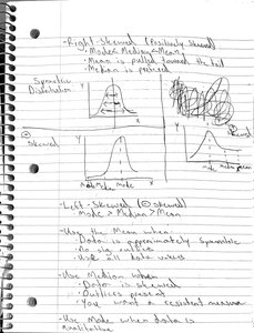
Skewness
Skewness describes the asymmetry of a distribution.
Right-skewed (positively skewed): Mean > Median > Mode
Left-skewed (negatively skewed): Mode > Median > Mean
Symmetric: Mean ≈ Median ≈ Mode
Correlation and Regression
Correlation
Correlation measures the strength and direction of a linear relationship between two variables.
Pearson Product-Moment Correlation:
Formula:
Types of Correlation:
Perfect positive (r = +1)
Perfect negative (r = -1)
No linear correlation (r = 0)
Regression
Regression analysis estimates the relationship between variables, often to predict one variable based on another.
Linear Regression: Fits a straight line to data points.
Equation:
Coefficient of Determination (R2): Measures the proportion of variance in y explained by x.
Probability
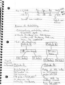
Basics of Probability
Probability quantifies the likelihood of events occurring. It is foundational for inferential statistics.
Probability Formula:
Simple Events: Outcomes that cannot be broken down further.
Compound Events: Outcomes composed of two or more simple events.
Percentiles and Z-Scores
Percentiles
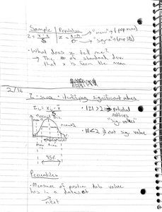
Percentiles indicate the position of a data value within a dataset.
Percentile Formula:
Z-Scores
Z-scores measure how many standard deviations a data value is from the mean.
Z-Score Formula:
Used to identify outliers and compare values across distributions.
Data Types and Classification
Quantitative vs. Categorical Data
Data can be classified as quantitative (numerical) or categorical (qualitative).
Quantitative:
Discrete: Countable values (e.g., number of students).
Continuous: Measurable values (e.g., height, weight).
Categorical:
Nominal: Categories without order (e.g., colors).
Ordinal: Categories with order (e.g., rankings).
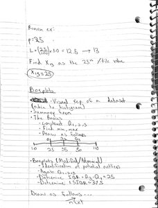
Boxplots
Visualizing Data Distribution
Boxplots provide a visual summary of data, showing the median, quartiles, and potential outliers.
Components:
Minimum, Q1, Median, Q3, Maximum
Outliers: Values outside 1.5 IQR from quartiles
Summary Table: Data Types
Type | Description | Examples |
|---|---|---|
Quantitative (Discrete) | Countable values | Number of books |
Quantitative (Continuous) | Measurable values | Height, weight |
Categorical (Nominal) | No order | Colors, gender |
Categorical (Ordinal) | Ordered categories | Rankings, grades |
Summary Table: Measures of Center
Measure | Definition | Properties |
|---|---|---|
Mean | Arithmetic average | Influenced by outliers |
Median | Middle value | Resistant to outliers |
Mode | Most frequent value | May not exist or may not be unique |
Summary Table: Measures of Variation
Measure | Definition | Properties |
|---|---|---|
Range | Max - Min | Simple, sensitive to outliers |
Variance | Average squared deviation | Units squared |
Standard Deviation | Square root of variance | Same units as data |
IQR | Q3 - Q1 | Resistant to outliers |
