Frequency Distributions for Organizing and Summarizing Data

Definition and Purpose

Frequency distributions are fundamental tools in statistics for organizing and summarizing large data sets. They help to reveal the distribution and patterns within the data, making it easier to interpret and analyze.

• Frequency Distribution: A table that displays the frequency, or count, of data values within specified intervals (called classes).

• Class Limits: The smallest and largest values that belong to each class.

• Class Boundaries: The values that separate classes without gaps.

• Class Width: The difference between the upper and lower boundaries of a class.

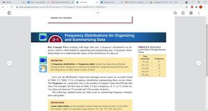
Example Table: Frequency Distribution

Constructing a Frequency Distribution

To construct a frequency distribution, follow these steps:

1. Determine the range of the data.

2. Choose the number of classes.

3. Calculate class width:

4. Set class limits and boundaries.

5. Tally the data into classes and count frequencies.

Histograms

Definition and Structure

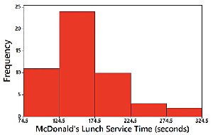
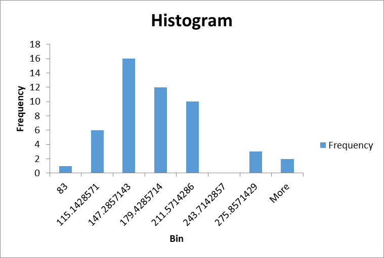
A histogram is a graphical representation of a frequency distribution. It consists of adjacent bars, where the horizontal axis represents class intervals and the vertical axis represents frequencies.

• Bars: Equal width, adjacent unless there are gaps in the data.

• Horizontal Scale: Quantitative data values (class intervals).

• Vertical Scale: Frequency values.

Important Uses of a Histogram

• Visually displays the shape of the data distribution.

• Shows the center of the data.

• Illustrates the spread (variation) of the data.

• Helps identify outliers.

Relative Frequency Histogram

A relative frequency histogram is similar to a standard histogram, but the vertical axis shows relative frequencies (proportions) instead of absolute counts. This allows for comparison between data sets of different sizes.

Interpreting Histograms: CVDOT

Critical Thinking: CVDOT

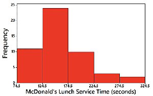
When analyzing histograms, consider the following aspects:

• Center: Where is the middle of the data?

• Variation: How spread out is the data?

• Distribution: What is the shape of the data?

• Outliers: Are there any unusual values?

• Time: Is there a time component or trend?

Common Distribution Shapes

Types of Distribution Shapes

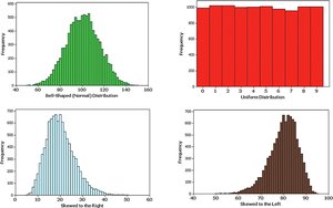
Histograms can reveal different shapes of data distributions, each with distinct characteristics:

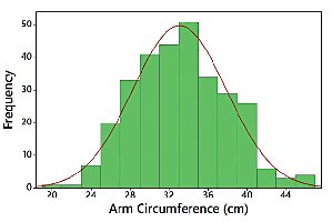
• Bell-Shaped (Normal) Distribution: Symmetric, with most values clustered around the center.

• Uniform Distribution: All values are equally likely; bars are of similar height.

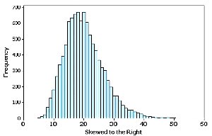
• Skewed Right: Longer tail on the right side; most values are on the left.

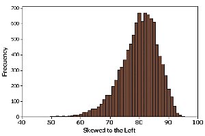
• Skewed Left: Longer tail on the left side; most values are on the right.

Normal Distribution

Characteristics of Normal Distribution

A normal distribution is a symmetric, bell-shaped curve. It is a fundamental concept in statistics, representing many natural phenomena.

• Mean, median, and mode are all equal.

• Most data values are close to the mean.

• Probability calculations often assume normality.

Skewness

Definition and Types

Skewness describes the asymmetry of a distribution. A distribution is skewed if it is not symmetric and extends more to one side.

• Skewed Right (Positive Skew): Longer tail on the right; mean > median.

• Skewed Left (Negative Skew): Longer tail on the left; mean < median.

Detecting Skewness by Comparing Mean and Median

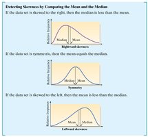
Skewness can be detected by comparing the mean and median:

• If the data set is symmetric, mean equals median.

• If skewed right, mean is greater than median.

• If skewed left, mean is less than median.

Using Excel to Construct Histograms

Excel’s Automatic Bins and Manual Bin Selection

Excel can be used to construct histograms efficiently. It offers automatic bin selection, but bins can also be manually adjusted for more precise analysis.

• Insert data into Excel worksheet.

• Select data and use the 'Insert' tab to choose 'Recommended Charts' or 'Histogram'.

• Adjust bin settings as needed for clarity.

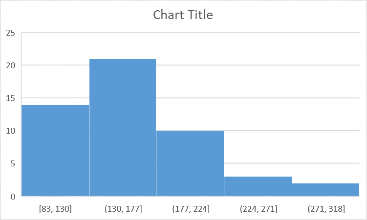
Example: Creating a Histogram in Excel

Follow these steps to create a histogram:

1. Enter data into a column.

2. Select the data.

3. Go to 'Insert' > 'Recommended Charts' > 'Histogram'.

4. Adjust bin width and labels as needed.

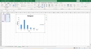
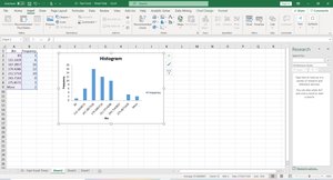
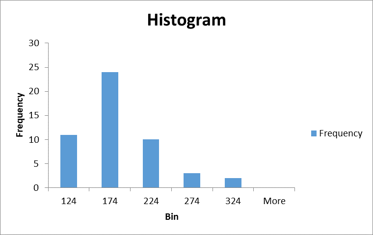
Summary Table: Distribution Shapes and Properties

Conclusion

Histograms and frequency distributions are essential for visualizing and understanding data in statistics. They provide insight into the shape, center, spread, and outliers of data sets, and tools like Excel make their construction accessible and efficient.