Organizing Qualitative Data

Frequency and Relative Frequency Distributions

Qualitative data, also known as categorical data, can be organized using frequency and relative frequency distributions. These tables help summarize the number of occurrences for each category and the proportion of the total each category represents.

• Frequency Distribution: Lists each category and the count of observations in each.

• Relative Frequency Distribution: Lists each category and the proportion (or percent) of observations in each, calculated as:

• Example: If 12 out of 30 patients require back rehabilitation, the relative frequency is or 40%.

Bar Graphs and Pareto Charts

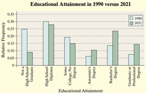
Bar graphs visually display the frequency or relative frequency of categories. Each bar represents a category, and the height corresponds to its frequency or relative frequency. Pareto charts are bar graphs with bars ordered from highest to lowest frequency.

• Bar Graph: Bars do not touch; used for qualitative data.

• Pareto Chart: Bars are arranged in decreasing order of frequency.

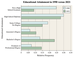
• Side-by-Side Bar Graphs: Used to compare two or more groups across the same categories, often using relative frequencies for fair comparison.

• Horizontal Bar Graphs: Useful when category names are long.

Pie Charts

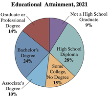
A pie chart is a circular graph divided into sectors, where each sector represents a category. The area of each sector is proportional to the category's frequency or relative frequency.

• Construction: Each sector's angle is calculated as .

• Example: If 9% of a population are not high school graduates, the sector for this group is .

Organizing Quantitative Data: The Popular Displays

Discrete vs. Continuous Data

Quantitative data can be discrete (countable values) or continuous (measurable values within an interval). The method of organization depends on the type of data:

• Discrete Data: If few values, use the values as categories; if many, group into intervals.

• Continuous Data: Always grouped into intervals (classes).

Frequency Distributions for Quantitative Data

For both discrete and continuous data, frequency and relative frequency distributions summarize the data. For continuous data, classes are defined by intervals with equal width (except in open-ended tables).

• Class Limits: Lower class limit is the smallest value in a class; upper class limit is the largest.

• Class Width: (rounded up).

• Open-Ended Tables: First or last class may lack a lower or upper limit.

Histograms

A histogram is a graphical representation of the frequency or relative frequency of quantitative data. Rectangles are drawn for each class, with heights representing frequency and widths equal for all classes. For continuous data, rectangles touch each other.

• Difference from Bar Graphs: In histograms, bars touch; in bar graphs, they do not.

Dot Plots

Dot plots display each data value as a dot above its corresponding value on a number line. Useful for small data sets to show distribution and clusters.

Identifying the Shape of a Distribution

The shape of a distribution can be described as:

• Uniform: All values occur with roughly equal frequency.

• Bell-Shaped (Normal): Highest frequency in the middle, tails off symmetrically.

• Skewed Right: Tail on the right is longer.

• Skewed Left: Tail on the left is longer.

Note: These terms are not used for qualitative data.

Additional Displays of Quantitative Data

Stem-and-Leaf Plots

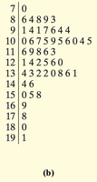
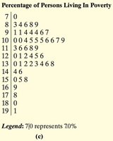
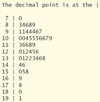
Stem-and-leaf plots display quantitative data while preserving the original values. The stem consists of all but the rightmost digit; the leaf is the rightmost digit. Leaves are listed in ascending order for each stem.

• Advantage: Raw data can be recovered from the plot.

• Split Stems: Used when data are bunched, splitting intervals for better visualization.

Frequency Polygons

A frequency polygon is a line graph that uses points connected by line segments to represent class frequencies. Points are plotted at class midpoints, and the graph is closed by connecting to the horizontal axis at each end.

• Class Midpoint:

Cumulative Frequency and Relative Frequency Tables

Cumulative frequency tables show the total number of observations less than or equal to each class. Cumulative relative frequency tables show the proportion (or percent) of observations less than or equal to each class.

Ogives

An ogive is a graph of cumulative frequency or cumulative relative frequency. Points are plotted at the upper class limits, and line segments connect the points. The graph starts at the horizontal axis at the lower end.

Time-Series Graphs

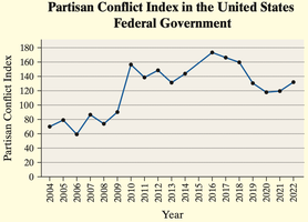
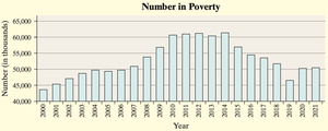
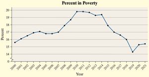
Time-series graphs display data collected over time. The horizontal axis represents time, and the vertical axis represents the variable measured. Line segments connect the data points to show trends.

Graphical Misrepresentations of Data

Common Ways Graphs Mislead

• Improper Category Definitions: Combining or splitting categories can distort interpretation.

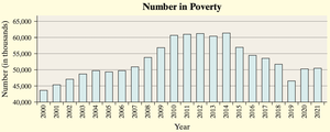
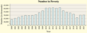
• Manipulating Vertical Scale: Not starting the vertical axis at zero exaggerates differences.

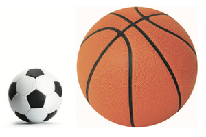
• Using Area or Volume Incorrectly: Pictograms or 3D graphs can misrepresent proportions.

• Clutter and Unclear Labels: Excessive decoration or missing labels confuse the reader.

Guidelines for Constructing Good Graphics

• Title and label axes clearly, including units and data sources.

• Avoid distortion and minimize white space.

• Indicate truncated scales with symbols.

• Avoid clutter and unnecessary 3D effects.

• Use consistent design and include data values or scales.