Chapter 2: Organizing Data

2.1 Variables and Data

In statistics, understanding the types of variables and data is foundational for proper data analysis. Variables are characteristics that can vary among individuals or items in a study.

• Variable: A characteristic that varies from one person or thing to another.

• Qualitative variable: A variable with non-numerical values (e.g., color, type, category).

• Quantitative variable: A variable with numerical values (e.g., height, weight, age).

• Discrete variable: A quantitative variable with countable, listed values (e.g., number of children).

• Continuous variable: A quantitative variable with values forming an interval on the real number line (e.g., temperature, time).

• Data: Information obtained by observing or measuring values of a variable.

Data are classified in the same way as variables: qualitative, quantitative discrete, and quantitative continuous.

2.2 Organizing Qualitative Data

To make sense of qualitative data, we organize and summarize it using tables and graphs.

• Frequency distribution (table): Lists distinct values and their frequencies (counts).

• Relative frequency distribution (table): Lists distinct values and their relative frequencies (proportions or percentages). The sum of relative frequencies should equal 1 (or 100%).

• Pie chart: A circular chart divided into wedges, where each wedge's size is proportional to the relative frequency of a category. There are 360 degrees in a circle. To find the angle for a category:

• Bar chart: Displays categories on the horizontal axis and frequencies (or relative frequencies/percentages) on the vertical axis. Bars do not touch for qualitative data.

All charts and graphs should be clearly labeled with a title, axis labels, and a numerical scale.

2.3 Organizing Quantitative Data

Quantitative data are often grouped into classes or categories to simplify analysis and visualization.

• Single-value grouping: Used for discrete data with a small number of distinct values.

• Limit grouping: Used for whole-number data with too many distinct values for single-value grouping.

• Cutpoint grouping: Used for continuous data, especially when values include decimals.

After grouping, create a table with frequencies, relative frequencies, or percentages for each group.

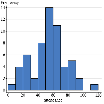
Histogram: A bar graph for quantitative data. Classes are on the horizontal axis, and frequencies (or relative frequencies/percentages) are on the vertical axis. Bars touch each other to indicate continuous data.

• Frequency histogram: Shows counts per class.

• Relative frequency histogram: Shows proportions per class.

• Percentage histogram: Shows percentages per class.

2.4 Distribution Shapes

The shape of a data distribution provides insight into the nature of the data. Common characteristics include symmetry, skewness, and modality.

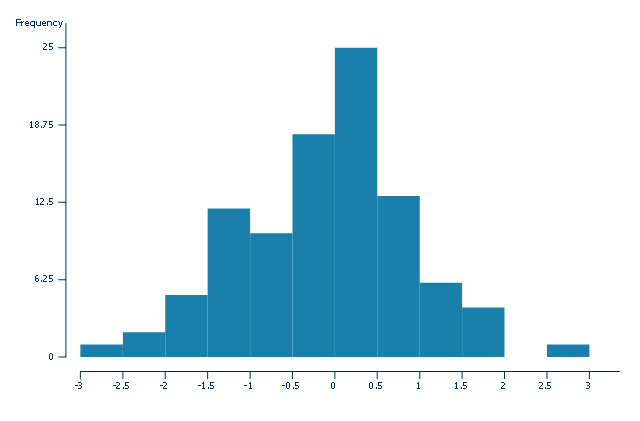
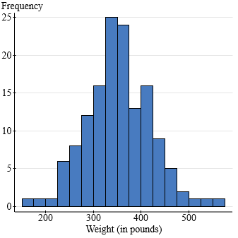
• Symmetric distribution: The left and right sides are mirror images.

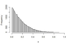
• Skewed distribution: The data stretch more to one side. Right-skewed (tail to the right), left-skewed (tail to the left).

• Modality: Refers to the number of peaks (modes) in the distribution (unimodal, bimodal, multimodal).

Examples of Distribution Shapes

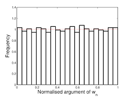
• Uniform distribution: All values are equally likely.

• Bell-shaped (normal) distribution: Symmetric with a single peak in the center.

• Right-skewed distribution: Most data are on the left, with a long tail to the right.

• Left-skewed distribution: Most data are on the right, with a long tail to the left.

Dot Plots and Stem-and-Leaf Diagrams

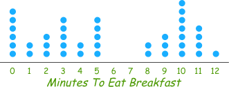
Dot plot: A simple way to display individual data points along a number line. Useful for small data sets.

Stem-and-leaf diagram: Displays actual data values while showing the distribution's shape. Stems are leading digits, leaves are final digits. Ordered diagrams sort leaves; two lines per stem can be used for clarity with larger data sets.

Population vs. Sample Distributions

Population data: Data from every individual in the group of interest.

Sample data: Data from a subset of the population.

Population distribution: The distribution of a variable for the entire population.

Sample distribution: The distribution of a variable for a sample. There is only one population distribution, but many possible sample distributions.

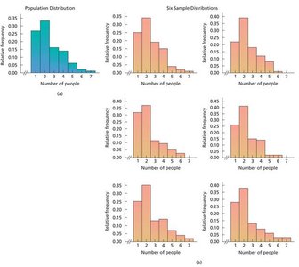
Key Fact: For a simple random sample, the sample distribution approximates the population distribution. Larger samples provide better approximations.

2.5 Misleading Graphs

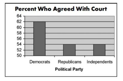
Graphs can be misleading if not constructed properly. Common issues include:

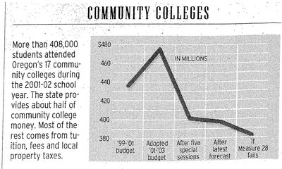
• Non-uniform scales

• Omitting zero from the axis

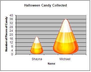
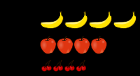
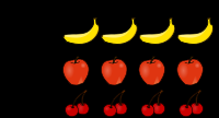
• Using images or shapes that exaggerate differences

• Improper labeling or lack of context

Best Practices for Graphs and Charts

• Always include a clear title.

• Label all axes and provide a uniform scale.

• Use appropriate types of graphs for the data (e.g., bars not touching for qualitative data, bars touching for quantitative data).

• Indicate breaks on axes where appropriate.