 Indietro
Regression, Correlation, and Residual Analysis in Introductory Statistics
Guida di studio - Note intelligenti
 Appunti personalizzati basati sui tuoi materiali, ampliati con definizioni chiave, esempi e contesto.
Regression and Correlation
Simple Linear Regression
Simple linear regression is a statistical method used to model the relationship between two quantitative variables. The model predicts the value of a dependent variable (response) based on the value of an independent variable (predictor).
Regression Equation: The general form is , where is the intercept and is the slope.
Interpretation of Slope (): The slope represents the average change in the response variable for each one-unit increase in the predictor variable.
Interpretation of Intercept (): The intercept is the predicted value of the response variable when the predictor variable is zero. In some contexts, this may not make practical sense.
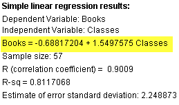
Example: For the regression equation Books = -0.688 + 1.5498 × Classes, the slope means that for each additional class, the expected number of books increases by about 1.55. The intercept suggests that with zero classes, the expected number of books is -0.688, which is not meaningful in this context.
Scatterplots and Line of Best Fit
A scatterplot visually displays the relationship between two quantitative variables. The line of best fit (regression line) summarizes this relationship.
Equation:
Purpose: To make predictions and understand the association between variables.
Correlation Coefficient (r)
The correlation coefficient, , measures the strength and direction of the linear relationship between two variables.
Range:
Interpretation: Values close to 1 or -1 indicate a strong linear relationship; values near 0 indicate a weak or no linear relationship.
Formula:
Coefficient of Determination ()
The coefficient of determination, , is the square of the correlation coefficient. It represents the proportion of the variance in the response variable that is explained by the predictor variable.
Range:
Interpretation: An of 0.81 means 81% of the variation in the response variable is explained by the model.
Conditions for Regression
Assumptions and Diagnostics
Before using a regression model, certain conditions must be checked:
Quantitative Variables: Both variables must be quantitative.
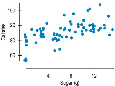
Straight Enough Condition: The scatterplot should show a linear pattern.
Outlier Condition: Outliers can have a large effect on the regression line.
Does the Plot Thicken? The spread of residuals should be roughly constant across all values of x.
Residuals and Residual Analysis
Definition and Interpretation
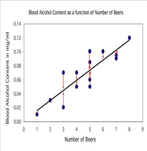
Residuals are the differences between observed and predicted values: .
Purpose: To assess the fit of the regression model.
Interpretation: Positive residuals indicate underprediction; negative residuals indicate overprediction.
Sum of Residuals: Always equals zero for least squares regression.
Residual Plots
A residual plot displays residuals on the vertical axis and the explanatory variable on the horizontal axis. It helps diagnose non-linearity, unequal error variances, and outliers.
Good Model: Residuals are randomly scattered around zero.
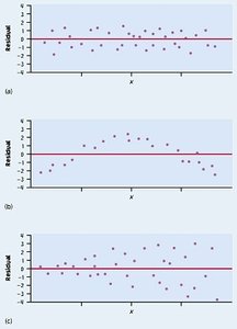
Problems: Patterns, bends, or changes in spread indicate issues with the model.
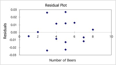
Examples of Residual Plots
Random Scatter: Indicates a good fit.
Curved Pattern: Suggests non-linearity.
Changing Spread: Indicates non-constant variance (heteroscedasticity).
Standard Deviation of Residuals ()
The standard deviation of the residuals, , measures the typical size of the prediction errors.
Interpretation: Smaller indicates more accurate predictions.
Outliers, Leverage, and Influence
Outliers
Outliers are points that fall outside the overall pattern of the data. They can affect the regression line and correlation.
Not all extreme values are outliers in the context of the relationship.
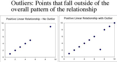
Leverage and Influence
Leverage: Points with extreme x-values have high leverage and can potentially affect the regression line.
Influential Points: Outliers that, if removed, significantly change the regression results (slope, , ).
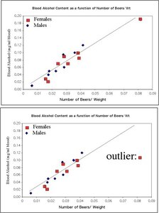
Interpreting Regression Results
Contextual Interpretation
Slope: Describes how the response variable tends to differ between groups or values, not how an individual will change.
Intercept: Only meaningful if x = 0 is within the scope of the data and makes sense contextually.
Prediction: Use the regression equation to predict y for a given x within the observed range.
Extrapolation: Avoid making predictions outside the range of observed x-values.
Limitations of Regression Analysis
Lurking Variables and Causation
Lurking Variable: A variable not included in the analysis that affects both the explanatory and response variables, possibly creating a spurious association.
Causation: Regression analysis alone cannot establish causation. Association does not imply causation.
Summary Table: Regression Output Interpretation
Statistic | Meaning |
|---|---|
Slope () | Average change in y for a one-unit increase in x |
Intercept () | Predicted y when x = 0 (context-dependent) |
Correlation (r) | Strength and direction of linear relationship |
R-squared () | Proportion of variance in y explained by x |
Standard error () | Typical prediction error |
Example Regression Outputs
Equation | r | R-sq | Interpretation |
|---|---|---|---|
Books = -0.688 + 1.5498 × Classes | 0.9009 | 0.8117 | Strong positive association; each class adds ~1.55 books |
Price = 17673.97 - 844.46 × Age | -0.8674 | 0.7524 | Older cars are worth less; strong negative association |
Weight = -195.74 + 4.99 × Height | 0.6440 | 0.4148 | Taller people tend to weigh more; moderate association |
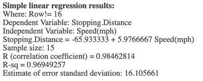
Stopping Distance = -169.52 + 8.85 × Speed | 0.9353 | 0.8747 | Higher speed increases stopping distance; very strong association |
