 Indietro
Sampling Distributions: Mean and Proportion (Chapter 8 Study Guide)
Guida di studio - Note intelligenti
 Appunti personalizzati basati sui tuoi materiali, ampliati con definizioni chiave, esempi e contesto.
Sampling Distributions
Introduction to Sampling Distributions
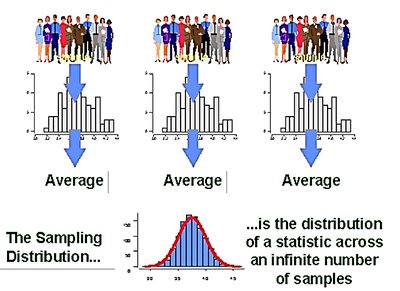
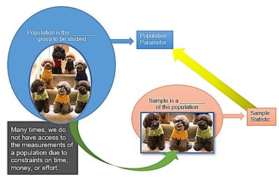
The concept of a sampling distribution is fundamental in statistics. It refers to the probability distribution of a given statistic (such as the mean or proportion) calculated from a random sample of size n drawn from a population. Understanding sampling distributions allows statisticians to make inferences about populations based on sample data.
Statistic: A numerical summary calculated from a sample.
Sampling Distribution: The distribution of a statistic across an infinite number of samples from the same population.
Population Parameter: A numerical summary describing the entire population.
Distribution of the Sample Mean, \( \bar{X} \)
Definition and Properties
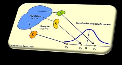
The sampling distribution of the sample mean \( \bar{X} \) is the probability distribution of all possible values of \( \bar{X} \) computed from samples of size n from a population with mean \( \mu \) and standard deviation \( \sigma \).
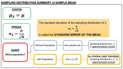
Center: The mean of the sampling distribution of \( \bar{X} \) is equal to the population mean \( \mu \).
Spread: The standard deviation of the sampling distribution (called the standard error) is \( \sigma_{\bar{X}} = \frac{\sigma}{\sqrt{n}} \).
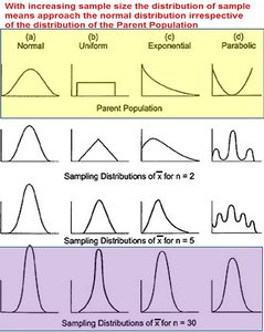
Shape: If the population is normal, the sampling distribution is normal for any sample size. If the population is not normal, the sampling distribution becomes approximately normal as sample size increases (Central Limit Theorem).
Example: IQ Scores (Normal Population)
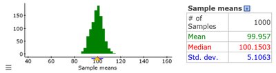
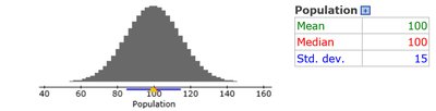
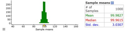
IQ scores are normally distributed with mean 100 and standard deviation 15. When many samples of size 9 are taken, the distribution of sample means is also normal, centered at 100, but with reduced spread.
Population: \( \mu = 100, \sigma = 15 \)
Sample Means: \( n = 9 \)
Effect of Sample Size
As sample size increases, the sampling distribution of the mean becomes more concentrated around the population mean, and its standard error decreases.
For \( n = 25 \), the spread of sample means is even smaller.
Example: MLB Salaries (Non-Normal Population)
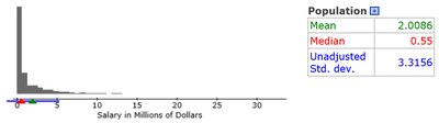
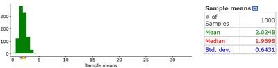
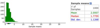
MLB salaries are highly skewed. Even with a non-normal population, the sampling distribution of the mean becomes approximately normal as sample size increases, illustrating the Central Limit Theorem.
Population: Skewed right, mean ≈ 2.01, std. dev. ≈ 3.32
Sample Means: For \( n = 9 \) and \( n = 25 \), the distribution of sample means becomes less skewed and more normal as \( n \) increases.
Central Limit Theorem (CLT)
The Central Limit Theorem states that the sampling distribution of the sample mean \( \bar{X} \) becomes approximately normal as the sample size increases, regardless of the population's shape. A sample size of at least 30 is typically sufficient for normality.
Rule of Thumb: \( n \geq 30 \) for approximate normality.
Standard Error of the Mean
The standard error quantifies the spread of the sampling distribution of the mean:
Formula:
As sample size increases, standard error decreases.
Practice Problems: Applications
Several problems illustrate the use of sampling distributions in real-world contexts:
IQ Scores: Calculating probabilities for individual and sample mean IQs.
Oil Change Facility: Estimating probabilities for mean oil-change times and setting performance goals.
Computer Repair Shop: Calculating the probability that mean daily revenue exceeds a threshold.


Distribution of the Sample Proportion, \( \hat{p} \)
Definition and Properties
The sample proportion \( \hat{p} \) is the ratio of individuals in a sample with a specified characteristic to the total sample size. It estimates the population proportion \( p \).
Formula:
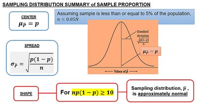
Center: The mean of the sampling distribution of \( \hat{p} \) is \( p \).
Spread: The standard deviation is
Shape: For large enough sample sizes (\( np(1-p) \geq 10 \)), the sampling distribution is approximately normal.
Examples: Estimating Population Proportion
Point estimates for population proportion are calculated from sample data:
Musicians: 368 out of 2540 are left-handed.
Households: 73 out of 250 own a snow blower.
Accidents: 44 out of 100 drivers at fault were inadequately insured.
Sampling Distribution of \( \hat{p} \): Applications
Problems illustrate the calculation of probabilities and the assessment of unusual events using the sampling distribution of the sample proportion:
Gallup survey: Probability that sample proportion exceeds a threshold.
Credit card ownership: Probability that sample proportion falls within a range.
Summary Table: Sampling Distribution of Sample Proportion
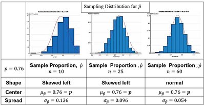
Sample Proportion, \( \hat{p} \) | n = 10 | n = 25 | n = 60 |
|---|---|---|---|
Shape | Skewed left | Skewed left | Normal |
Center | \( \mu_{\hat{p}} = p = 0.76 \) | \( \mu_{\hat{p}} = p = 0.76 \) | \( \mu_{\hat{p}} = p = 0.76 \) |
Spread | \( \sigma_{\hat{p}} = 0.136 \) | \( \sigma_{\hat{p}} = 0.096 \) | \( \sigma_{\hat{p}} = 0.054 \) |

Summary Table: Sampling Distribution of Sample Proportion (General)
Property | Formula | Condition |
|---|---|---|
Center | \( \mu_{\hat{p}} = p \) | -- |
Spread | \( \sigma_{\hat{p}} = \sqrt{ \frac{p(1-p)}{n} } \) | Sample size \( \leq 0.05N \) |
Shape | Approximately normal | \( np(1-p) \geq 10 \) |

Key Takeaways
Sampling distributions allow inference about population parameters from sample statistics.
The Central Limit Theorem ensures normality of the sampling distribution of the mean for large samples.
Sample proportions estimate population proportions, and their sampling distributions are approximately normal for large samples.
Standard error quantifies the variability of sample means or proportions.
