Scatterplots, Correlation, and Regression

Introduction to Paired Data Analysis

In statistics, analyzing paired sample data helps us understand the relationship between two quantitative variables. This section introduces the concepts of correlation and regression, focusing on how to visualize and quantify associations using scatterplots, the linear correlation coefficient, and regression lines.

Scatterplots

A scatterplot (or scatter diagram) is a graphical representation of paired quantitative data. Each point on the plot corresponds to one observation, with the horizontal axis (x-axis) representing the first variable and the vertical axis (y-axis) representing the second variable. Scatterplots are essential for visually assessing the relationship between two variables.

• Purpose: To visually detect patterns, trends, or associations between variables.

• Interpretation: Patterns in the scatterplot may suggest the presence or absence of a relationship.

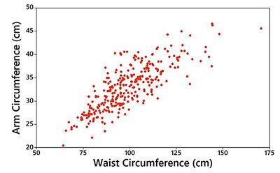
Example: The scatterplot above shows a clear pattern, indicating a correlation between waist and arm circumferences.

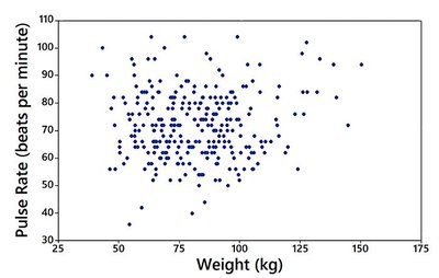
Example: The scatterplot above shows no distinct pattern, suggesting no correlation between weight and pulse rate.

Correlation

Correlation measures the degree to which two variables are related. Specifically, a linear correlation exists when the relationship between variables can be approximated by a straight line.

• Positive Correlation: As one variable increases, the other tends to increase.

• Negative Correlation: As one variable increases, the other tends to decrease.

• No Correlation: No discernible pattern or association between the variables.

Linear Correlation Coefficient (r)

The linear correlation coefficient, denoted by r, quantifies the strength and direction of a linear relationship between two variables. The value of r ranges from -1 to 1:

• r = 1: Perfect positive linear correlation

• r = -1: Perfect negative linear correlation

• r = 0: No linear correlation

• Interpretation: Values of r close to -1 or 1 indicate strong correlation; values near 0 indicate weak or no linear correlation.

Formula for r:

Additional info: The formula above is the Pearson correlation coefficient for paired data (x, y).

Examples: Correlation in Practice

Consider the relationship between shoe print length and height:

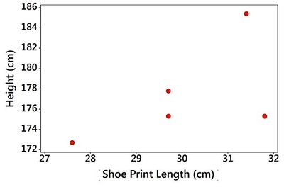
With a small sample size (n = 5), it is difficult to determine if a linear correlation exists.

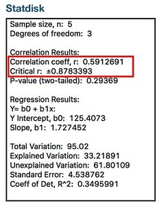
The computed correlation coefficient is r = 0.591, with a P-value of 0.294. This high P-value suggests that the observed correlation could easily occur by chance, so there is not enough evidence to conclude a linear correlation exists.

P-Value in Correlation Analysis

The P-value in correlation analysis is the probability of obtaining a correlation coefficient as extreme as the observed value, assuming there is no actual linear correlation in the population.

• Small P-value (≤ 0.05): Indicates strong evidence against the null hypothesis (no correlation); supports the existence of a linear correlation.

• Large P-value (> 0.05): Indicates insufficient evidence to conclude a linear correlation exists.

Example: For n = 5, r = 0.591, P-value = 0.294. Since 0.294 > 0.05, we do not conclude a linear correlation exists.

Effect of Sample Size

With a larger sample size (n = 40), the relationship between shoe print length and height becomes clearer:

Here, r = 0.813 and P-value = 0.000, indicating a strong, statistically significant linear correlation.

Regression and the Regression Line

Regression is a statistical method for modeling the relationship between two variables by fitting a straight line (the regression line or line of best fit) to the data. The regression equation describes this line algebraically:

• \( \hat{y} \): Predicted value of the dependent variable

• \( b_0 \): y-intercept (value of \( \hat{y} \) when x = 0)

• \( b_1 \): Slope (change in \( \hat{y} \) for a one-unit increase in x)

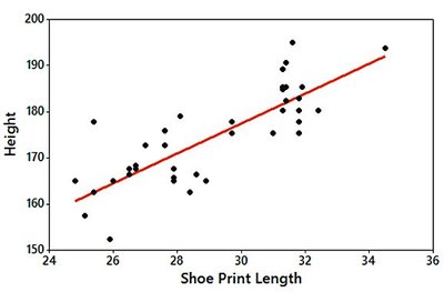
Example: For the shoe print length and height data, the regression equation is:

This means that for each additional centimeter in shoe print length, the predicted height increases by 3.22 cm.

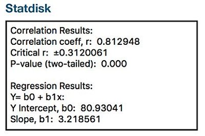
Additional info: The regression output provides the y-intercept (b0 = 80.9) and slope (b1 = 3.22), matching the regression equation above.

Summary Table: Correlation and Regression Interpretation