Normal Distribution

Definition and Properties

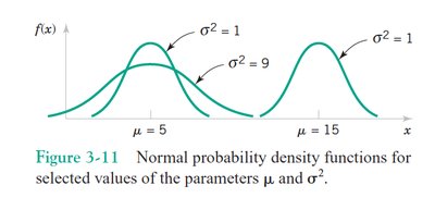
The normal distribution is a fundamental probability distribution in statistics, characterized by its symmetric, bell-shaped curve. It is used to model many natural phenomena and measurement errors. The distribution is defined by two parameters: the mean (\(\mu\)) and the standard deviation (\(\sigma\)).

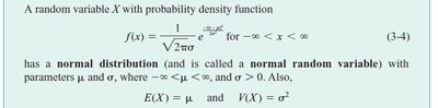
• Probability Density Function (PDF): The normal distribution for a random variable \(X\) is given by: where \(-\infty < x < \infty\), \(-\infty < \mu < \infty\), and \(\sigma > 0\).

• Mean: \(E(X) = \mu\)

• Variance: \(V(X) = \sigma^2\)

• Shape: The curve is symmetric about the mean, and the spread is determined by the standard deviation.

The Empirical Rule

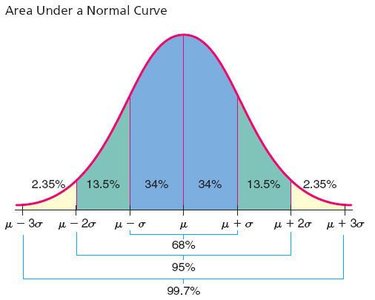
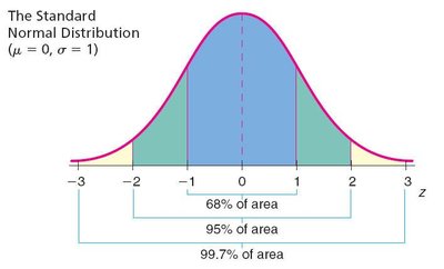
The Empirical Rule describes the proportion of data within certain intervals of the mean in a normal distribution:

• Approximately 68% of values lie within one standard deviation (\(\mu \pm \sigma\))

• Approximately 95% of values lie within two standard deviations (\(\mu \pm 2\sigma\))

• Approximately 99.7% of values lie within three standard deviations (\(\mu \pm 3\sigma\))

Standard Normal Distribution

Definition

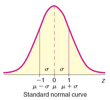
The standard normal distribution is a special case of the normal distribution with mean \(\mu = 0\) and variance \(\sigma^2 = 1\). It is denoted by the random variable \(Z\).

• Standard normal random variable: \(Z\)

• Mean: \(0\)

• Variance: \(1\)

Z-Score and Standardization

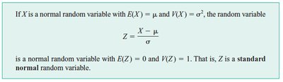
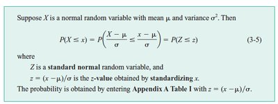
A z-score is a standardized value that indicates how many standard deviations a data point is from the mean. Standardizing allows comparison across different normal distributions.

• Formula for z-score:

• After standardization, \(Z\) has mean 0 and variance 1.

Areas Under the Normal Curve

Cumulative Distribution Function (CDF)

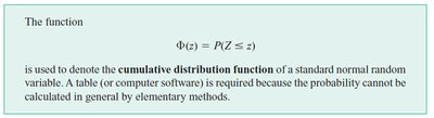
The cumulative distribution function (CDF) for the standard normal variable \(Z\) is denoted as \(\Phi(z) = P(Z \leq z)\). It gives the probability that \(Z\) is less than or equal to a given value.

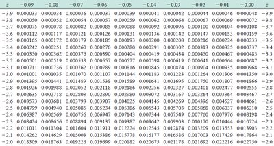
• Probabilities are found using tables or software, as there is no simple closed-form solution.

Finding Probabilities Using Z-Tables

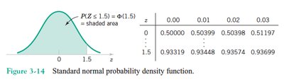
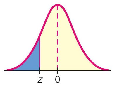
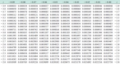
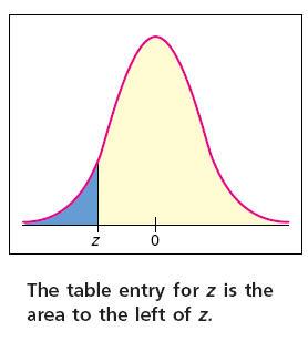
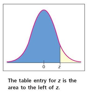
Z-tables provide the area under the standard normal curve to the left of a given z-score. This area represents the probability \(P(Z \leq z)\).

• To find \(P(Z \leq z)\), locate z in the table.

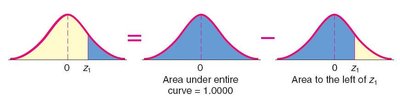
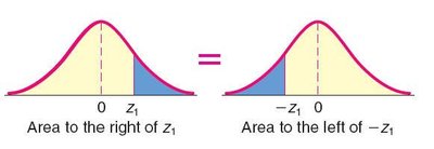
• To find \(P(Z > z)\), subtract the area to the left of z from 1:

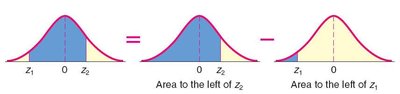
• To find the area between two z-values, subtract the area to the left of the lower z from the area to the left of the higher z:

Inverse Normal Probability Distribution

Finding Z or X Values for Given Areas

Sometimes, it is necessary to find the z-score or original x-value that corresponds to a specified area (probability) under the normal curve. This is known as the inverse normal probability problem.

• For a left-tail area \(A\), find z such that \(P(Z \leq z) = A\).

• For a right-tail area \(A\), find z such that \(P(Z > z) = A\), or equivalently \(P(Z \leq z) = 1 - A\).

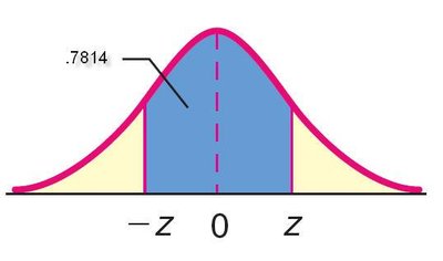
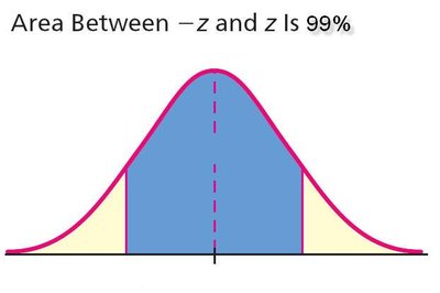
• For a symmetric center area \(A\), find \(\pm z\) such that \(P(-z < Z < z) = A\).

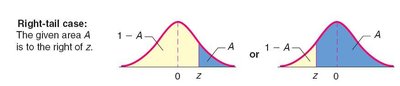
Examples and Applications

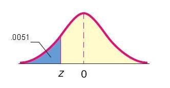
• Example: If the area to the left of z is 0.0051, then z is approximately -2.58.

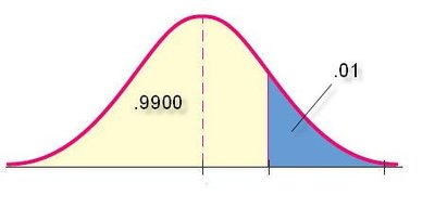
• Example: If the area to the right of z is 0.01, then z is approximately 2.33.

• Example: If the area between -z and z is 0.7814, then z is approximately 1.15.

• Example: Area between -z and z is 99%.

• Example: Area between -z and z is 95%.

Summary Table: Normal Distribution Concepts

Key Takeaways

• The normal distribution is central to statistical inference and probability.

• Standardization allows comparison and calculation of probabilities using z-tables.

• Areas under the curve represent probabilities and are used for hypothesis testing, confidence intervals, and more.