Summarizing and Graphing Data

Introduction to Summarizing and Graphing Data

Summarizing and graphing data are essential steps in statistics that help us understand, interpret, and communicate information from raw data sets. This chapter focuses on organizing data into tables and visual representations to reveal patterns, trends, and relationships.

Frequency Distributions

Definition and Purpose

A frequency distribution is a table that displays how a data set is partitioned among several classes (intervals), listing each class and the number of values (frequency) in each class. Frequency distributions help organize data for easier analysis and pattern recognition.

• Does not maintain original data values—only the count per class.

• Useful for both quantitative and categorical (qualitative) data.

Parts of a Frequency Distribution

• Frequency: The number of values in a class.

• Lower Class Limit: The smallest number that can belong to a class.

• Upper Class Limit: The largest number that can belong to a class.

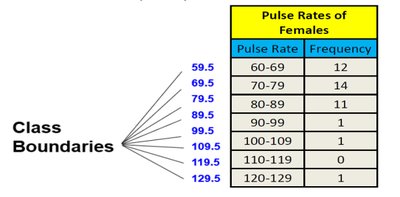
• Class Boundaries: Numbers used to separate classes without gaps.

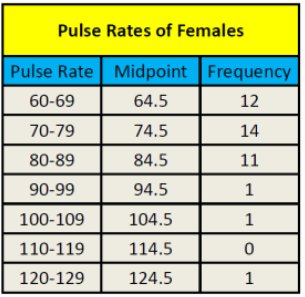
• Class Midpoint: The value in the middle of a class, calculated as the average of the lower and upper class limits.

• Class Width: The difference between consecutive lower (or upper) class limits. All classes should have the same width.

Constructing a Frequency Distribution

1. Sort the data and determine the number of classes (usually between 5 and 20).

2. Calculate class width using the formula:

3. Choose the minimum data value as the first lower class limit.

4. List all lower and upper class limits using the class width.

5. Count the frequency for each class.

6. Include titles, labels, and optionally midpoints and relative frequencies.

Example: Frequency Distribution

Suppose we have the pulse rates (beats per minute) of 40 females:

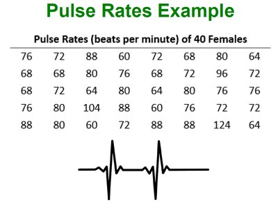
The frequency distribution for these data might look like:

Relative and Cumulative Frequency Distributions

Relative Frequency Distribution

A relative frequency is the proportion (or percentage) of data values in each class, calculated as:

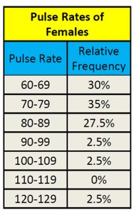
Cumulative Frequency Distribution

A cumulative frequency is the sum of the frequencies for that class and all previous classes. It shows how many data values are less than the upper boundary of each class.

Graphical Representations of Data

Dot Plots

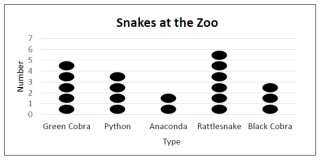
A dot plot displays individual data values as dots along a number line. Dots representing equal values are stacked. Dot plots are useful for both quantitative and categorical data.

Histograms

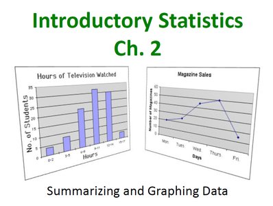
A histogram is a bar graph for quantitative data where the horizontal axis represents classes and the vertical axis represents frequencies. Histograms do not retain original data values but show the distribution's shape.

Relative Frequency Histogram

Similar to a histogram, but the vertical axis shows relative frequencies (percentages) instead of counts.

Frequency Polygon

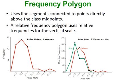
A frequency polygon uses line segments to connect points directly above class midpoints at heights corresponding to class frequencies. A relative frequency polygon uses relative frequencies for the vertical scale.

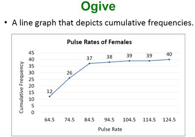
Ogive

An ogive is a line graph that depicts cumulative frequencies. It helps visualize how many data values are below a particular value.

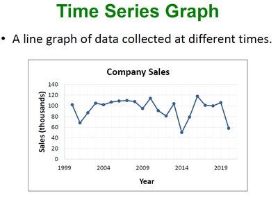
Time Series Graph

A time series graph is a line graph of data collected at different points in time, useful for identifying trends over time.

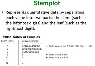
Stemplot (Stem-and-Leaf Plot)

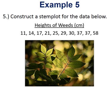
A stemplot represents quantitative data by splitting each value into a "stem" (all but the rightmost digit) and a "leaf" (the rightmost digit). This plot retains original data values and shows distribution shape.

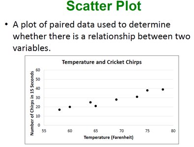
Scatter Plot

A scatter plot is a graph of paired data (x, y) used to determine if there is a relationship between two variables. Each point represents a pair of values.

Analyzing Graphs and Common Errors

Shape of Distributions

• Symmetric: The left and right sides of the histogram are approximately mirror images.

• Skewed: The distribution is not symmetric; it may be skewed left (tail on the left) or right (tail on the right).

Graph Construction Errors

• Choosing an inappropriate graph type for the data

• Omitting titles, labels, or scales

• Misrepresenting data by distorting axes or intervals

All graphs should be clear, accurate, and appropriate for the data type.

Summary Table: Types of Frequency Distributions

Key Formulas

• Class Width:

• Class Midpoint:

• Relative Frequency:

• Cumulative Frequency:

Conclusion

Summarizing and graphing data are foundational skills in statistics. By organizing data into tables and visual displays, we can better understand distributions, identify trends, and communicate findings effectively. Mastery of these techniques is essential for further study in statistics and data analysis.