Normal Probability Distributions

Standard Normal Distribution

The standard normal distribution is a special case of the normal distribution with a mean of 0 and a standard deviation of 1. It is used extensively in statistics to calculate probabilities and critical values for hypothesis testing and confidence intervals.

• Mean (μ): 0

• Standard Deviation (σ): 1

• Notation: Z ~ N(0, 1)

The standard normal distribution is symmetric about the mean, and the total area under the curve is 1.

Z-Scores

A z-score indicates how many standard deviations a value is from the mean. It is calculated as:

• X: The value from the dataset

• μ: The mean of the distribution

• σ: The standard deviation of the distribution

Z-scores allow us to compare values from different normal distributions and to find probabilities using the standard normal table.

Using the Standard Normal Table

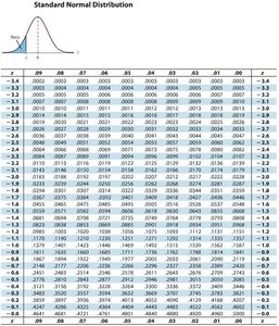
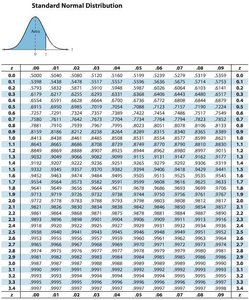
The standard normal table (also called the z-table) provides the area (probability) to the left of a given z-score in the standard normal distribution. This area represents the cumulative probability up to that z-score.

• Rows correspond to the integer and first decimal place of the z-score (e.g., 1.2).

• Columns correspond to the second decimal place (e.g., .03).

• Find the intersection to get the cumulative probability.

Example: Finding Probabilities

Example: What is the probability that Z < 1.23?

1. Locate 1.2 in the leftmost column.

2. Move across to the column labeled .03.

3. The value at the intersection is the probability: P(Z < 1.23).

Suppose the table value is 0.8907. Thus, P(Z < 1.23) = 0.8907.

Finding Areas to the Right or Between Values

• To find P(Z > z): Subtract the table value from 1.

• To find P(a < Z < b): Subtract the table value for a from the table value for b.

Example: P(Z > 1.23) = 1 - 0.8907 = 0.1093

Example: P(0.5 < Z < 1.2) = P(Z < 1.2) - P(Z < 0.5)

Table Structure and Interpretation

The standard normal table is structured as follows:

Additional info: Table values are cumulative probabilities from the far left up to the given z-score. For negative z-scores, use symmetry: P(Z < -z) = 1 - P(Z < z).

Applications in Statistics

• Finding probabilities for normal distributions

• Calculating p-values in hypothesis testing

• Constructing confidence intervals

• Standardizing data for comparison